Suvarna Garge (Editor)

Linear regression

Updated on
Edit
Like
Comment
Share on FacebookTweet on TwitterShare on LinkedInShare on Reddit
Linear regression

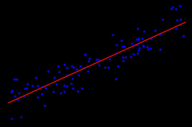
In statistics, linear regression is an approach for modeling the relationship between a scalar dependent variable y and one or more explanatory variables (or independent variables) denoted X. The case of one explanatory variable is called simple linear regression. For more than one explanatory variable, the process is called multiple linear regression. (This term is distinct from multivariate linear regression, where multiple correlated dependent variables are predicted, rather than a single scalar variable.)

Contents

In linear regression, the relationships are modeled using linear predictor functions whose unknown model parameters are estimated from the data. Such models are called linear models. Most commonly, the conditional mean of y given the value of X is assumed to be an affine function of X; less commonly, the median or some other quantile of the conditional distribution of y given X is expressed as a linear function of X. Like all forms of regression analysis, linear regression focuses on the conditional probability distribution of y given X, rather than on the joint probability distribution of y and X, which is the domain of multivariate analysis.

Linear regression was the first type of regression analysis to be studied rigorously, and to be used extensively in practical applications. This is because models which depend linearly on their unknown parameters are easier to fit than models which are non-linearly related to their parameters and because the statistical properties of the resulting estimators are easier to determine.

Linear regression has many practical uses. Most applications fall into one of the following two broad categories:

  • If the goal is prediction, or forecasting, or error reduction, linear regression can be used to fit a predictive model to an observed data set of y and X values. After developing such a model, if an additional value of X is then given without its accompanying value of y, the fitted model can be used to make a prediction of the value of y.
  • Given a variable y and a number of variables X1, ..., Xp that may be related to y, linear regression analysis can be applied to quantify the strength of the relationship between y and the Xj, to assess which Xj may have no relationship with y at all, and to identify which subsets of the Xj contain redundant information about y.
  • Linear regression models are often fitted using the least squares approach, but they may also be fitted in other ways, such as by minimizing the "lack of fit" in some other norm (as with least absolute deviations regression), or by minimizing a penalized version of the least squares loss function as in ridge regression (L2-norm penalty) and lasso (L1-norm penalty). Conversely, the least squares approach can be used to fit models that are not linear models. Thus, although the terms "least squares" and "linear model" are closely linked, they are not synonymous.

    Introduction

    Given a data set { y i , x i 1 , , x i p } i = 1 n of n statistical units, a linear regression model assumes that the relationship between the dependent variable yi and the p-vector of regressors xi is linear. This relationship is modeled through a disturbance term or error variable εi — an unobserved random variable that adds noise to the linear relationship between the dependent variable and regressors. Thus the model takes the form

    y i = β 1 x i 1 + + β p x i p + ε i = x i T β + ε i , i = 1 , , n ,

    where T denotes the transpose, so that xiTβ is the inner product between vectors xi and β.

    Often these n equations are stacked together and written in vector form as

    y = X β + ε ,

    where

    y = ( y 1 y 2 y n ) , X = ( x 1 T x 2 T x n T ) = ( x 11 x 1 p x 21 x 2 p x n 1 x n p ) , β = ( β 1 β 2 β p ) , ε = ( ε 1 ε 2 ε n ) .

    Some remarks on terminology and general use:

  • y i is called the regressand, endogenous variable, response variable, measured variable, criterion variable, or dependent variable (see dependent and independent variables). The decision as to which variable in a data set is modeled as the dependent variable and which are modeled as the independent variables may be based on a presumption that the value of one of the variables is caused by, or directly influenced by the other variables. Alternatively, there may be an operational reason to model one of the variables in terms of the others, in which case there need be no presumption of causality.
  • x i 1 , x i 2 , , x i p are called regressors, exogenous variables, explanatory variables, covariates, input variables, predictor variables, or independent variables (see dependent and independent variables, but not to be confused with independent random variables). The matrix X is sometimes called the design matrix.
  • Usually a constant is included as one of the regressors. For example, we can take xi1 = 1 for i = 1, ..., n. The corresponding element of β is called the intercept. Many statistical inference procedures for linear models require an intercept to be present, so it is often included even if theoretical considerations suggest that its value should be zero.
  • Sometimes one of the regressors can be a non-linear function of another regressor or of the data, as in polynomial regression and segmented regression. The model remains linear as long as it is linear in the parameter vector β.
  • The regressors xij may be viewed either as random variables, which we simply observe, or they can be considered as predetermined fixed values which we can choose. Both interpretations may be appropriate in different cases, and they generally lead to the same estimation procedures; however different approaches to asymptotic analysis are used in these two situations.
  • β is a p-dimensional parameter vector. Its elements are also called effects, or regression coefficients. Statistical estimation and inference in linear regression focuses on β. The elements of this parameter vector are interpreted as the partial derivatives of the dependent variable with respect to the various independent variables.
  • ε i is called the error term, disturbance term, or noise. This variable captures all other factors which influence the dependent variable yi other than the regressors xi. The relationship between the error term and the regressors, for example whether they are correlated, is a crucial step in formulating a linear regression model, as it will determine the method to use for estimation.
  • Example. Consider a situation where a small ball is being tossed up in the air and then we measure its heights of ascent hi at various moments in time ti. Physics tells us that, ignoring the drag, the relationship can be modeled as

    h i = β 1 t i + β 2 t i 2 + ε i ,

    where β1 determines the initial velocity of the ball, β2 is proportional to the standard gravity, and εi is due to measurement errors. Linear regression can be used to estimate the values of β1 and β2 from the measured data. This model is non-linear in the time variable, but it is linear in the parameters β1 and β2; if we take regressors xi = (xi1, xi2)  = (ti, ti2), the model takes on the standard form

    h i = x i T β + ε i .

    Assumptions

    Standard linear regression models with standard estimation techniques make a number of assumptions about the predictor variables, the response variables and their relationship. Numerous extensions have been developed that allow each of these assumptions to be relaxed (i.e. reduced to a weaker form), and in some cases eliminated entirely. Some methods are general enough that they can relax multiple assumptions at once, and in other cases this can be achieved by combining different extensions. Generally these extensions make the estimation procedure more complex and time-consuming, and may also require more data in order to produce an equally precise model.

    The following are the major assumptions made by standard linear regression models with standard estimation techniques (e.g. ordinary least squares):

  • Weak exogeneity. This essentially means that the predictor variables x can be treated as fixed values, rather than random variables. This means, for example, that the predictor variables are assumed to be error-free—that is, not contaminated with measurement errors. Although this assumption is not realistic in many settings, dropping it leads to significantly more difficult errors-in-variables models.
  • Linearity. This means that the mean of the response variable is a linear combination of the parameters (regression coefficients) and the predictor variables. Note that this assumption is much less restrictive than it may at first seem. Because the predictor variables are treated as fixed values (see above), linearity is really only a restriction on the parameters. The predictor variables themselves can be arbitrarily transformed, and in fact multiple copies of the same underlying predictor variable can be added, each one transformed differently. This trick is used, for example, in polynomial regression, which uses linear regression to fit the response variable as an arbitrary polynomial function (up to a given rank) of a predictor variable. This makes linear regression an extremely powerful inference method. In fact, models such as polynomial regression are often "too powerful", in that they tend to overfit the data. As a result, some kind of regularization must typically be used to prevent unreasonable solutions coming out of the estimation process. Common examples are ridge regression and lasso regression. Bayesian linear regression can also be used, which by its nature is more or less immune to the problem of overfitting. (In fact, ridge regression and lasso regression can both be viewed as special cases of Bayesian linear regression, with particular types of prior distributions placed on the regression coefficients.)
  • Constant variance (a.k.a. homoscedasticity). This means that different response variables have the same variance in their errors, regardless of the values of the predictor variables. In practice this assumption is invalid (i.e. the errors are heteroscedastic) if the response variables can vary over a wide scale. In order to determine for heterogeneous error variance, or when a pattern of residuals violates model assumptions of homoscedasticity (error is equally variable around the 'best-fitting line' for all points of x), it is prudent to look for a "fanning effect" between residual error and predicted values. This is to say there will be a systematic change in the absolute or squared residuals when plotted against the predicting outcome. Error will not be evenly distributed across the regression line. Heteroscedasticity will result in the averaging over of distinguishable variances around the points to get a single variance that is inaccurately representing all the variances of the line. In effect, residuals appear clustered and spread apart on their predicted plots for larger and smaller values for points along the linear regression line, and the mean squared error for the model will be wrong. Typically, for example, a response variable whose mean is large will have a greater variance than one whose mean is small. For example, a given person whose income is predicted to be $100,000 may easily have an actual income of $80,000 or $120,000 (a standard deviation of around $20,000), while another person with a predicted income of $10,000 is unlikely to have the same $20,000 standard deviation, which would imply their actual income would vary anywhere between -$10,000 and $30,000. (In fact, as this shows, in many cases—often the same cases where the assumption of normally distributed errors fails—the variance or standard deviation should be predicted to be proportional to the mean, rather than constant.) Simple linear regression estimation methods give less precise parameter estimates and misleading inferential quantities such as standard errors when substantial heteroscedasticity is present. However, various estimation techniques (e.g. weighted least squares and heteroscedasticity-consistent standard errors) can handle heteroscedasticity in a quite general way. Bayesian linear regression techniques can also be used when the variance is assumed to be a function of the mean. It is also possible in some cases to fix the problem by applying a transformation to the response variable (e.g. fit the logarithm of the response variable using a linear regression model, which implies that the response variable has a log-normal distribution rather than a normal distribution).
  • Independence of errors. This assumes that the errors of the response variables are uncorrelated with each other. (Actual statistical independence is a stronger condition than mere lack of correlation and is often not needed, although it can be exploited if it is known to hold.) Some methods (e.g. generalized least squares) are capable of handling correlated errors, although they typically require significantly more data unless some sort of regularization is used to bias the model towards assuming uncorrelated errors. Bayesian linear regression is a general way of handling this issue.
  • Lack of multicollinearity in the predictors. For standard least squares estimation methods, the design matrix X must have full column rank p; otherwise, we have a condition known as multicollinearity in the predictor variables. This can be triggered by having two or more perfectly correlated predictor variables (e.g. if the same predictor variable is mistakenly given twice, either without transforming one of the copies or by transforming one of the copies linearly). It can also happen if there is too little data available compared to the number of parameters to be estimated (e.g. fewer data points than regression coefficients). In the case of multicollinearity, the parameter vector β will be non-identifiable—it has no unique solution. At most we will be able to identify some of the parameters, i.e. narrow down its value to some linear subspace of Rp. See partial least squares regression. Methods for fitting linear models with multicollinearity have been developed; some require additional assumptions such as "effect sparsity"—that a large fraction of the effects are exactly zero.
    Note that the more computationally expensive iterated algorithms for parameter estimation, such as those used in generalized linear models, do not suffer from this problem—and in fact it's quite normal when handling categorically valued predictors to introduce a separate indicator variable predictor for each possible category, which inevitably introduces multicollinearity.
  • Beyond these assumptions, several other statistical properties of the data strongly influence the performance of different estimation methods:

  • The statistical relationship between the error terms and the regressors plays an important role in determining whether an estimation procedure has desirable sampling properties such as being unbiased and consistent.
  • The arrangement, or probability distribution of the predictor variables x has a major influence on the precision of estimates of β. Sampling and design of experiments are highly developed subfields of statistics that provide guidance for collecting data in such a way to achieve a precise estimate of β.
  • Interpretation

    A fitted linear regression model can be used to identify the relationship between a single predictor variable xj and the response variable y when all the other predictor variables in the model are "held fixed". Specifically, the interpretation of βj is the expected change in y for a one-unit change in xj when the other covariates are held fixed—that is, the expected value of the partial derivative of y with respect to xj. This is sometimes called the unique effect of xj on y. In contrast, the marginal effect of xj on y can be assessed using a correlation coefficient or simple linear regression model relating xj to y; this effect is the total derivative of y with respect to xj.

    Care must be taken when interpreting regression results, as some of the regressors may not allow for marginal changes (such as dummy variables, or the intercept term), while others cannot be held fixed (recall the example from the introduction: it would be impossible to "hold ti fixed" and at the same time change the value of ti2).

    It is possible that the unique effect can be nearly zero even when the marginal effect is large. This may imply that some other covariate captures all the information in xj, so that once that variable is in the model, there is no contribution of xj to the variation in y. Conversely, the unique effect of xj can be large while its marginal effect is nearly zero. This would happen if the other covariates explained a great deal of the variation of y, but they mainly explain variation in a way that is complementary to what is captured by xj. In this case, including the other variables in the model reduces the part of the variability of y that is unrelated to xj, thereby strengthening the apparent relationship with xj.

    The meaning of the expression "held fixed" may depend on how the values of the predictor variables arise. If the experimenter directly sets the values of the predictor variables according to a study design, the comparisons of interest may literally correspond to comparisons among units whose predictor variables have been "held fixed" by the experimenter. Alternatively, the expression "held fixed" can refer to a selection that takes place in the context of data analysis. In this case, we "hold a variable fixed" by restricting our attention to the subsets of the data that happen to have a common value for the given predictor variable. This is the only interpretation of "held fixed" that can be used in an observational study.

    The notion of a "unique effect" is appealing when studying a complex system where multiple interrelated components influence the response variable. In some cases, it can literally be interpreted as the causal effect of an intervention that is linked to the value of a predictor variable. However, it has been argued that in many cases multiple regression analysis fails to clarify the relationships between the predictor variables and the response variable when the predictors are correlated with each other and are not assigned following a study design. A commonality analysis may be helpful in disentangling the shared and unique impacts of correlated independent variables.

    Extensions

    Numerous extensions of linear regression have been developed, which allow some or all of the assumptions underlying the basic model to be relaxed.

    Simple and multiple regression

    The very simplest case of a single scalar predictor variable x and a single scalar response variable y is known as simple linear regression. The extension to multiple and/or vector-valued predictor variables (denoted with a capital X) is known as multiple linear regression, also known as multivariable linear regression. Nearly all real-world regression models involve multiple predictors, and basic descriptions of linear regression are often phrased in terms of the multiple regression model. Note, however, that in these cases the response variable y is still a scalar. Another term multivariate linear regression refers to cases where y is a vector, i.e., the same as general linear regression.

    General linear models

    The general linear model considers the situation when the response variable Y is not a scalar but a vector. Conditional linearity of E(y|x) = Bx is still assumed, with a matrix B replacing the vector β of the classical linear regression model. Multivariate analogues of Ordinary Least-Squares (OLS) and Generalized Least-Squares (GLS) have been developed. "General linear models" are also called "multivariate linear models". These are not the same as multivariable linear models (also called "multiple linear models").

    Heteroscedastic models

    Various models have been created that allow for heteroscedasticity, i.e. the errors for different response variables may have different variances. For example, weighted least squares is a method for estimating linear regression models when the response variables may have different error variances, possibly with correlated errors. (See also Weighted linear least squares, and Generalized least squares.) Heteroscedasticity-consistent standard errors is an improved method for use with uncorrelated but potentially heteroscedastic errors.

    Generalized linear models

    Generalized linear models (GLMs) are a framework for modeling a response variable y that is bounded or discrete. This is used, for example:

  • when modeling positive quantities (e.g. prices or populations) that vary over a large scale—which are better described using a skewed distribution such as the log-normal distribution or Poisson distribution (although GLMs are not used for log-normal data, instead the response variable is simply transformed using the logarithm function);
  • when modeling categorical data, such as the choice of a given candidate in an election (which is better described using a Bernoulli distribution/binomial distribution for binary choices, or a categorical distribution/multinomial distribution for multi-way choices), where there are a fixed number of choices that cannot be meaningfully ordered;
  • when modeling ordinal data, e.g. ratings on a scale from 0 to 5, where the different outcomes can be ordered but where the quantity itself may not have any absolute meaning (e.g. a rating of 4 may not be "twice as good" in any objective sense as a rating of 2, but simply indicates that it is better than 2 or 3 but not as good as 5).
  • Generalized linear models allow for an arbitrary link function g that relates the mean of the response variable to the predictors, i.e. E(y) = g(βx). The link function is often related to the distribution of the response, and in particular it typically has the effect of transforming between the ( , ) range of the linear predictor and the range of the response variable.

    Some common examples of GLMs are:

  • Poisson regression for count data.
  • Logistic regression and probit regression for binary data.
  • Multinomial logistic regression and multinomial probit regression for categorical data.
  • Ordered probit regression for ordinal data.
  • Single index models allow some degree of nonlinearity in the relationship between x and y, while preserving the central role of the linear predictor βx as in the classical linear regression model. Under certain conditions, simply applying OLS to data from a single-index model will consistently estimate β up to a proportionality constant.

    Hierarchical linear models

    Hierarchical linear models (or multilevel regression) organizes the data into a hierarchy of regressions, for example where A is regressed on B, and B is regressed on C. It is often used where the variables of interest have a natural hierarchical structure such as in educational statistics, where students are nested in classrooms, classrooms are nested in schools, and schools are nested in some administrative grouping, such as a school district. The response variable might be a measure of student achievement such as a test score, and different covariates would be collected at the classroom, school, and school district levels.

    Errors-in-variables

    Errors-in-variables models (or "measurement error models") extend the traditional linear regression model to allow the predictor variables X to be observed with error. This error causes standard estimators of β to become biased. Generally, the form of bias is an attenuation, meaning that the effects are biased toward zero.

    Others

  • In Dempster–Shafer theory, or a linear belief function in particular, a linear regression model may be represented as a partially swept matrix, which can be combined with similar matrices representing observations and other assumed normal distributions and state equations. The combination of swept or unswept matrices provides an alternative method for estimating linear regression models.
  • Estimation methods

    A large number of procedures have been developed for parameter estimation and inference in linear regression. These methods differ in computational simplicity of algorithms, presence of a closed-form solution, robustness with respect to heavy-tailed distributions, and theoretical assumptions needed to validate desirable statistical properties such as consistency and asymptotic efficiency.

    Some of the more common estimation techniques for linear regression are summarized below.

  • Maximum likelihood estimation can be performed when the distribution of the error terms is known to belong to a certain parametric family ƒθ of probability distributions. When fθ is a normal distribution with zero mean and variance θ, the resulting estimate is identical to the OLS estimate. GLS estimates are maximum likelihood estimates when ε follows a multivariate normal distribution with a known covariance matrix.
  • Ridge regression, and other forms of penalized estimation such as Lasso regression, deliberately introduce bias into the estimation of β in order to reduce the variability of the estimate. The resulting estimators generally have lower mean squared error than the OLS estimates, particularly when multicollinearity is present or when overfitting is a problem. They are generally used when the goal is to predict the value of the response variable y for values of the predictors x that have not yet been observed. These methods are not as commonly used when the goal is inference, since it is difficult to account for the bias.
  • Least absolute deviation (LAD) regression is a robust estimation technique in that it is less sensitive to the presence of outliers than OLS (but is less efficient than OLS when no outliers are present). It is equivalent to maximum likelihood estimation under a Laplace distribution model for ε.
  • Adaptive estimation. If we assume that error terms are independent from the regressors ε i x i , the optimal estimator is the 2-step MLE, where the first step is used to non-parametrically estimate the distribution of the error term.
  • Other estimation techniques

  • Bayesian linear regression applies the framework of Bayesian statistics to linear regression. (See also Bayesian multivariate linear regression.) In particular, the regression coefficients β are assumed to be random variables with a specified prior distribution. The prior distribution can bias the solutions for the regression coefficients, in a way similar to (but more general than) ridge regression or lasso regression. In addition, the Bayesian estimation process produces not a single point estimate for the "best" values of the regression coefficients but an entire posterior distribution, completely describing the uncertainty surrounding the quantity. This can be used to estimate the "best" coefficients using the mean, mode, median, any quantile (see quantile regression), or any other function of the posterior distribution.
  • Quantile regression focuses on the conditional quantiles of y given X rather than the conditional mean of y given X. Linear quantile regression models a particular conditional quantile, for example the conditional median, as a linear function βTx of the predictors.
  • Mixed models are widely used to analyze linear regression relationships involving dependent data when the dependencies have a known structure. Common applications of mixed models include analysis of data involving repeated measurements, such as longitudinal data, or data obtained from cluster sampling. They are generally fit as parametric models, using maximum likelihood or Bayesian estimation. In the case where the errors are modeled as normal random variables, there is a close connection between mixed models and generalized least squares. Fixed effects estimation is an alternative approach to analyzing this type of data.
  • Principal component regression (PCR) is used when the number of predictor variables is large, or when strong correlations exist among the predictor variables. This two-stage procedure first reduces the predictor variables using principal component analysis then uses the reduced variables in an OLS regression fit. While it often works well in practice, there is no general theoretical reason that the most informative linear function of the predictor variables should lie among the dominant principal components of the multivariate distribution of the predictor variables. The partial least squares regression is the extension of the PCR method which does not suffer from the mentioned deficiency.
  • Least-angle regression is an estimation procedure for linear regression models that was developed to handle high-dimensional covariate vectors, potentially with more covariates than observations.
  • The Theil–Sen estimator is a simple robust estimation technique that chooses the slope of the fit line to be the median of the slopes of the lines through pairs of sample points. It has similar statistical efficiency properties to simple linear regression but is much less sensitive to outliers.
  • Other robust estimation techniques, including the α-trimmed mean approach, and L-, M-, S-, and R-estimators have been introduced.
  • Further discussion

    In statistics and numerical analysis, the problem of numerical methods for linear least squares is an important one because linear regression models are one of the most important types of model, both as formal statistical models and for exploration of data sets. The majority of statistical computer packages contain facilities for regression analysis that make use of linear least squares computations. Hence it is appropriate that considerable effort has been devoted to the task of ensuring that these computations are undertaken efficiently and with due regard to numerical precision.

    Individual statistical analyses are seldom undertaken in isolation, but rather are part of a sequence of investigatory steps. Some of the topics involved in considering numerical methods for linear least squares relate to this point. Thus important topics can be

  • Computations where a number of similar, and often nested, models are considered for the same data set. That is, where models with the same dependent variable but different sets of independent variables are to be considered, for essentially the same set of data points.
  • Computations for analyses that occur in a sequence, as the number of data points increases.
  • Special considerations for very extensive data sets.
  • Fitting of linear models by least squares often, but not always, arises in the context of statistical analysis. It can therefore be important that considerations of computational efficiency for such problems extend to all of the auxiliary quantities required for such analyses, and are not restricted to the formal solution of the linear least squares problem.

    Matrix calculations, like any others, are affected by rounding errors. An early summary of these effects, regarding the choice of computational methods for matrix inversion, was provided by Wilkinson.

    Using linear algebra

    It follows that one can find a "best" approximation of another function by minimizing the area between two functions, a continuous function f on [ a , b ] and a function g W where W is a subspace of C [ a , b ] :

    Area = a b | f ( x ) g ( x ) | d x ,

    all within the subspace W . Due to the frequent difficulty of evaluating integrands involving absolute value, one can instead define

    a b [ f ( x ) g ( x ) ] 2 d x

    as an adequate criterion for obtaining the least squares approximation, function g , of f with respect to the inner product space W .

    As such, f g 2 or, equivalently, f g , can thus be written in vector form:

    a b [ f ( x ) g ( x ) ] 2 d x = f g , f g = f g 2 .

    In other words, the least squares approximation of f is the function g  subspace  W closest to f in terms of the inner product f , g . Furthermore, this can be applied with a theorem:

    Let f be continuous on [ a , b ] , and let W be a finite-dimensional subspace of C [ a , b ] . The least squares approximating function of f with respect to W is given by g = f , w 1 w 1 + f , w 2 w 2 + + f , w n w n , where B = { w 1 , w 2 , , w n } is an orthonormal basis for W .

    Applications of linear regression

    Linear regression is widely used in biological, behavioral and social sciences to describe possible relationships between variables. It ranks as one of the most important tools used in these disciplines.

    Trend line

    A trend line represents a trend, the long-term movement in time series data after other components have been accounted for. It tells whether a particular data set (say GDP, oil prices or stock prices) have increased or decreased over the period of time. A trend line could simply be drawn by eye through a set of data points, but more properly their position and slope is calculated using statistical techniques like linear regression. Trend lines typically are straight lines, although some variations use higher degree polynomials depending on the degree of curvature desired in the line.

    Trend lines are sometimes used in business analytics to show changes in data over time. This has the advantage of being simple. Trend lines are often used to argue that a particular action or event (such as training, or an advertising campaign) caused observed changes at a point in time. This is a simple technique, and does not require a control group, experimental design, or a sophisticated analysis technique. However, it suffers from a lack of scientific validity in cases where other potential changes can affect the data.

    Epidemiology

    Early evidence relating tobacco smoking to mortality and morbidity came from observational studies employing regression analysis. In order to reduce spurious correlations when analyzing observational data, researchers usually include several variables in their regression models in addition to the variable of primary interest. For example, suppose we have a regression model in which cigarette smoking is the independent variable of interest, and the dependent variable is lifespan measured in years. Researchers might include socio-economic status as an additional independent variable, to ensure that any observed effect of smoking on lifespan is not due to some effect of education or income. However, it is never possible to include all possible confounding variables in an empirical analysis. For example, a hypothetical gene might increase mortality and also cause people to smoke more. For this reason, randomized controlled trials are often able to generate more compelling evidence of causal relationships than can be obtained using regression analyses of observational data. When controlled experiments are not feasible, variants of regression analysis such as instrumental variables regression may be used to attempt to estimate causal relationships from observational data.

    Finance

    The capital asset pricing model uses linear regression as well as the concept of beta for analyzing and quantifying the systematic risk of an investment. This comes directly from the beta coefficient of the linear regression model that relates the return on the investment to the return on all risky assets.

    Economics

    Linear regression is the predominant empirical tool in economics. For example, it is used to predict consumption spending, fixed investment spending, inventory investment, purchases of a country's exports, spending on imports, the demand to hold liquid assets, labor demand, and labor supply.

    Environmental science

    Linear regression finds application in a wide range of environmental science applications. In Canada, the Environmental Effects Monitoring Program uses statistical analyses on fish and benthic surveys to measure the effects of pulp mill or metal mine effluent on the aquatic ecosystem.

    References

    Linear regression Wikipedia