In statistics, errors-in-variables models or measurement error models are regression models that account for measurement errors in the independent variables. In contrast, standard regression models assume that those regressors have been measured exactly, or observed without error; as such, those models account only for errors in the dependent variables, or responses.
In the case when some regressors have been measured with errors, estimation based on the standard assumption leads to inconsistent estimates, meaning that the parameter estimates do not tend to the true values even in very large samples. For simple linear regression the effect is an underestimate of the coefficient, known as the attenuation bias. In non-linear models the direction of the bias is likely to be more complicated.
Consider a simple linear regression model of the form
y t = α + β x t ∗ + ε t , t = 1 , … , T , where x t ∗ denotes the true but unobserved regressor. Instead we observe this value with an error:
x t = x t ∗ + η t where the measurement error η t is assumed to be independent from the true value x t ∗ .
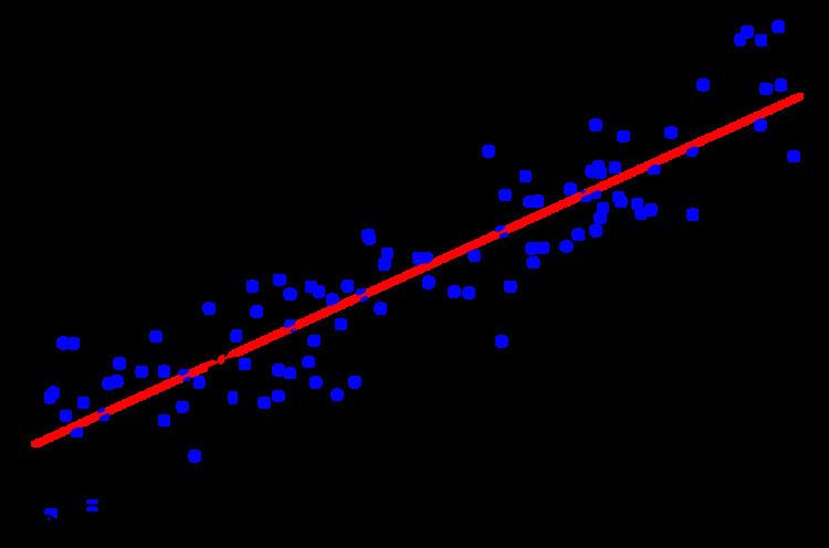
If the y t ′s are simply regressed on the x t ′s (see simple linear regression), then the estimator for the slope coefficient is
β ^ = 1 T ∑ t = 1 T ( x t − x ¯ ) ( y t − y ¯ ) 1 T ∑ t = 1 T ( x t − x ¯ ) 2 , which converges as the sample size T increases without bound:
β ^ → p Cov [ x t , y t ] Var [ x t ] = β σ x ∗ 2 σ x ∗ 2 + σ η 2 = β 1 + σ η 2 / σ x ∗ 2 . Variances are non-negative, so that in the limit the estimate is smaller in magnitude than the true value of β , an effect which statisticians call attenuation or regression dilution. Thus the ‘naїve’ least squares estimator is inconsistent in this setting. However, the estimator is a consistent estimator of the parameter required for a best linear predictor of y given x : in some applications this may be what is required, rather than an estimate of the ‘true’ regression coefficient, although that would assume that the variance of the errors in observing x ∗ remains fixed. This follows directly from the result quoted immediately above, and the fact that the regression coefficient relating the y t ′s to the actually observed x t ′s, in a simple linear regression, is given by
β x = Cov [ x t , y t ] Var [ x t ] . It is this coefficient, rather than β , that would be required for constructing a predictor of y based on an observed x which is subject to noise.
It can be argued that almost all existing data sets contain errors of different nature and magnitude, so that attenuation bias is extremely frequent (although in multivariate regression the direction of bias is ambiguous. Jerry Hausman sees this as an iron law of econometrics: "The magnitude of the estimate is usually smaller than expected."
Usually measurement error models are described using the latent variables approach. If y is the response variable and x are observed values of the regressors, then it is assumed there exist some latent variables y ∗ and x ∗ which follow the model's “true” functional relationship g ( ⋅ ) , and such that the observed quantities are their noisy observations:
{ x = x ∗ + η , y = y ∗ + ε , y ∗ = g ( x ∗ , w | θ ) , where θ is the model's parameter and w are those regressors which are assumed to be error-free (for example when linear regression contains an intercept, the regressor which corresponds to the constant certainly has no "measurement errors"). Depending on the specification these error-free regressors may or may not be treated separately; in the latter case it is simply assumed that corresponding entries in the variance matrix of η 's are zero.
The variables y , x , w are all observed, meaning that the statistician possesses a data set of n statistical units { y i , x i , w i } i = 1 , … , n which follow the data generating process described above; the latent variables x ∗ , y ∗ , ε , and η are not observed however.
This specification does not encompass all the existing errors-in-variables models. For example in some of them function g ( ⋅ ) may be non-parametric or semi-parametric. Other approaches model the relationship between y ∗ and x ∗ as distributional instead of functional, that is they assume that y ∗ conditionally on x ∗ follows a certain (usually parametric) distribution.
Terminology and assumptions
The observed variable x may be called the manifest, indicator, or proxy variable.The unobserved variable x ∗ may be called the latent or true variable. It may be regarded either as an unknown constant (in which case the model is called a functional model), or as a random variable (correspondingly a structural model).The relationship between the measurement error η and the latent variable x ∗ can be modeled in different ways:Classical errors: η ⊥ x ∗ the errors are independent from the latent variable. This is the most common assumption, it implies that the errors are introduced by the measuring device and their magnitude does not depend on the value being measured.Mean-independence: E [ η | x ∗ ] = 0 , the errors are mean-zero for every value of the latent regressor. This is a less restrictive assumption than the classical one, as it allows for the presence of heteroscedasticity or other effects in the measurement errors.Berkson's errors: η ⊥ x , the errors are independent from the observed regressor x. This assumption has very limited applicability. One example is round-off errors: for example if a person's age* is a continuous random variable, whereas the observed age is truncated to the next smallest integer, then the truncation error is approximately independent from the observed age. Another possibility is with the fixed design experiment: for example if a scientist decides to make a measurement at a certain predetermined moment of time x , say at x = 10 s , then the real measurement may occur at some other value of x ∗ (for example due to her finite reaction time) and such measurement error will be generally independent from the "observed" value of the regressor.Misclassification errors: special case used for the dummy regressors. If x ∗ is an indicator of a certain event or condition (such as person is male/female, some medical treatment given/not, etc.), then the measurement error in such regressor will correspond to the incorrect classification similar to type I and type II errors in statistical testing. In this case the error η may take only 3 possible values, and its distribution conditional on x ∗ is modeled with two parameters: α = Pr [ η = − 1 | x ∗ = 1 ] , and β = Pr [ η = 1 | x ∗ = 0 ] . The necessary condition for identification is that α + β < 1 , that is misclassification should not happen "too often". (This idea can be generalized to discrete variables with more than two possible values.)Linear errors-in-variables models were studied first, probably because linear models were so widely used and they are easier than non-linear ones. Unlike standard least squares regression (OLS), extending errors in variables regression (EiV) from the simple to the multivariable case is not straightforward.
The simple linear errors-in-variables model was already presented in the "motivation" section:
{ y t = α + β x t ∗ + ε t , x t = x t ∗ + η t , where all variables are scalar. Here α and β are the parameters of interest, whereas σε and ση—standard deviations of the error terms—are the nuisance parameters. The "true" regressor x* is treated as a random variable (structural model), independent from the measurement error η (classic assumption).
This model is identifiable in two cases: (1) either the latent regressor x* is not normally distributed, (2) or x* has normal distribution, but neither εt nor ηt are divisible by a normal distribution. That is, the parameters α, β can be consistently estimated from the data set ( x t , y t ) t = 1 T without any additional information, provided the latent regressor is not Gaussian.
Before this identifiability result was established, statisticians attempted to apply the maximum likelihood technique by assuming that all variables are normal, and then concluded that the model is not identified. The suggested remedy was to assume that some of the parameters of the model are known or can be estimated from the outside source. Such estimation methods include
Deming regression — assumes that the ratio δ = σ²ε/σ²η is known. This could be appropriate for example when errors in y and x are both caused by measurements, and the accuracy of measuring devices or procedures are known. The case when δ = 1 is also known as the orthogonal regression.Regression with known reliability ratio λ = σ²∗/ ( σ²η + σ²∗), where σ²∗ is the variance of the latent regressor. Such approach may be applicable for example when repeating measurements of the same unit are available, or when the reliability ratio has been known from the independent study. In this case the consistent estimate of slope is equal to the least-squares estimate divided by λ.Regression with known σ²η may occur when the source of the errors in x's is known and their variance can be calculated. This could include rounding errors, or errors introduced by the measuring device. When σ²η is known we can compute the reliability ratio as λ = ( σ²x − σ²η) / σ²x and reduce the problem to the previous case.Newer estimation methods that do not assume knowledge of some of the parameters of the model, include
Multivariable model looks exactly like the simple linear model, only this time β, ηt, xt and x*t are k×1 vectors.
{ y t = α + β ′ x t ∗ + ε t , x t = x t ∗ + η t . The general identifiability condition for this model remains an open question. It is known however that in the case when (ε,η) are independent and jointly normal, the parameter β is identified if and only if it is impossible to find a non-singular k×k block matrix [a A] (where a is a k×1 vector) such that a′x* is distributed normally and independently from A′x*.
Some of the estimation methods for multivariable linear models are
A generic non-linear measurement error model takes form
{ y t = g ( x t ∗ ) + ε t , x t = x t ∗ + η t . Here function g can be either parametric or non-parametric. When function g is parametric it will be written as g(x*, β).
For a general vector-valued regressor x* the conditions for model identifiability are not known. However in the case of scalar x* the model is identified unless the function g is of the "log-exponential" form
g ( x ∗ ) = a + b ln ( e c x ∗ + d ) and the latent regressor x* has density
f x ∗ ( x ) = { A e − B e C x + C D x ( e C x + E ) − F , if d > 0 A e − B x 2 + C x if d = 0 where constants A,B,C,D,E,F may depend on a,b,c,d.
Despite this optimistic result, as of now no methods exist for estimating non-linear errors-in-variables models without any extraneous information. However there are several techniques which make use of some additional data: either the instrumental variables, or repeated observations.
In this approach two (or maybe more) repeated observations of the regressor x* are available. Both observations contain their own measurement errors, however those errors are required to be independent:
{ x 1 t = x t ∗ + η 1 t , x 2 t = x t ∗ + η 2 t , where x* ⊥ η1 ⊥ η2. Variables η1, η2 need not be identically distributed (although if they are efficiency of the estimator can be slightly improved). With only these two observations it is possible to consistently estimate the density function of x* using Kotlarski's deconvolution technique.