Ordinary least squares

Linear model

Suppose the data consists of n observations { y
i, x
i }n
i=1. Each observation includes a scalar response y_i and a vector of p predictors (or regressors) x_i. In a linear regression model the response variable is a linear function of the regressors:

y i = x i T β + ε i ,

where β is a p×1 vector of unknown parameters; ε_i's are unobserved scalar random variables (errors) which account for the discrepancy between the actually observed responses y_i and the "predicted outcomes" x_i^Tβ; and ^T denotes matrix transpose, so that x^Tβ is the dot product between the vectors x and β. This model can also be written in matrix notation as

y = X β + ε ,

where y and ε are n×1 vectors, and X is an n×p matrix of regressors, which is also sometimes called the design matrix.

As a rule, the constant term is always included in the set of regressors X, say, by taking x_i1 = 1 for all i = 1, …, n. The coefficient β₁ corresponding to this regressor is called the intercept.

There may be some relationship between the regressors. For instance, the third regressor may be the square of the second regressor. In this case (assuming that the first regressor is constant) we have a quadratic model in the second regressor. But this is still considered a linear model because it is linear in the βs.

Assumptions

There are several different frameworks in which the linear regression model can be cast in order to make the OLS technique applicable. Each of these settings produces the same formulas and same results. The only difference is the interpretation and the assumptions which have to be imposed in order for the method to give meaningful results. The choice of the applicable framework depends mostly on the nature of data in hand, and on the inference task which has to be performed.

One of the lines of difference in interpretation is whether to treat the regressors as random variables, or as predefined constants. In the first case (random design) the regressors x_i are random and sampled together with the y_i's from some population, as in an observational study. This approach allows for more natural study of the asymptotic properties of the estimators. In the other interpretation (fixed design), the regressors X are treated as known constants set by a design, and y is sampled conditionally on the values of X as in an experiment. For practical purposes, this distinction is often unimportant, since estimation and inference is carried out while conditioning on X. All results stated in this article are within the random design framework.

Classical linear regression model

The classical model focuses on the "finite sample" estimation and inference, meaning that the number of observations n is fixed. This contrasts with the other approaches, which study the asymptotic behavior of OLS, and in which the number of observations is allowed to grow to infinity.

Correct specification. The linear functional form is correctly specified.

Strict exogeneity. The errors in the regression should have conditional mean zero: E ⁡ [ ε ∣ X ] = 0.

The immediate consequence of the exogeneity assumption is that the errors have mean zero: E[ε] = 0, and that the regressors are uncorrelated with the errors: E[X^Tε] = 0.The exogeneity assumption is critical for the OLS theory. If it holds then the regressor variables are called exogenous. If it doesn't, then those regressors that are correlated with the error term are called endogenous, and then the OLS estimates become invalid. In such case the method of instrumental variables may be used to carry out inference.

No linear dependence. The regressors in X must all be linearly independent. Mathematically, this means that the matrix X must have full column rank almost surely: Pr [ rank ⁡ ( X ) = p ] = 1.

Usually, it is also assumed that the regressors have finite moments up to at least the second moment. Then the matrix Q_xx = E[X^TX / n] is finite and positive semi-definite.When this assumption is violated the regressors are called linearly dependent or perfectly multicollinear. In such case the value of the regression coefficient β cannot be learned, although prediction of y values is still possible for new values of the regressors that lie in the same linearly dependent subspace.

Spherical errors: Var ⁡ [ ε ∣ X ] = σ 2 I n ,

where I_n is the identity matrix in dimension n, and σ² is a parameter which determines the variance of each observation. This σ² is considered a nuisance parameter in the model, although usually it is also estimated. If this assumption is violated then the OLS estimates are still valid, but no longer efficient.It is customary to split this assumption into two parts:

Homoscedasticity: E[ ε_i² | X ] = σ², which means that the error term has the same variance σ² in each observation. When this requirement is violated this is called heteroscedasticity, in such case a more efficient estimator would be weighted least squares. If the errors have infinite variance then the OLS estimates will also have infinite variance (although by the law of large numbers they will nonetheless tend toward the true values so long as the errors have zero mean). In this case, robust estimation techniques are recommended.

No autocorrelation: the errors are uncorrelated between observations: E[ ε_iε_j | X ] = 0 for i ≠ j. This assumption may be violated in the context of time series data, panel data, cluster samples, hierarchical data, repeated measures data, longitudinal data, and other data with dependencies. In such cases generalized least squares provides a better alternative than the OLS. Another expression for autocorrelation is serial correlation.

Normality. It is sometimes additionally assumed that the errors have normal distribution conditional on the regressors: ε ∣ X ∼ N ( 0 , σ 2 I n ) .

This assumption is not needed for the validity of the OLS method, although certain additional finite-sample properties can be established in case when it does (especially in the area of hypotheses testing). Also when the errors are normal, the OLS estimator is equivalent to the maximum likelihood estimator (MLE), and therefore it is asymptotically efficient in the class of all regular estimators. Importantly, the normality assumption applies only to the error terms; contrary to a popular misconception, the response (dependent) variable is not required to be normally distributed.

Independent and identically distributed (iid)

In some applications, especially with cross-sectional data, an additional assumption is imposed — that all observations are independent and identically distributed. This means that all observations are taken from a random sample which makes all the assumptions listed earlier simpler and easier to interpret. Also this framework allows one to state asymptotic results (as the sample size n → ∞), which are understood as a theoretical possibility of fetching new independent observations from the data generating process. The list of assumptions in this case is:

iid observations: (x_i, y_i) is independent from, and has the same distribution as, (x_j, y_j) for all i ≠ j;

no perfect multicollinearity: Q_xx = E[ x_i x_i^T ] is a positive-definite matrix;

exogeneity: E[ ε_i | x_i ] = 0;

homoscedasticity: Var[ ε_i | x_i ] = σ².

Time series model

The stochastic process {x_i, y_i} is stationary and ergodic;

The regressors are predetermined: E[x_iε_i] = 0 for all i = 1, …, n;

The p×p matrix Q_xx = E[ x_i x_i^T ] is of full rank, and hence positive-definite;

{x_iε_i} is a martingale difference sequence, with a finite matrix of second moments Q_xxε² = E[ ε_i²x_i x_i^T ].

Estimation

Suppose b is a "candidate" value for the parameter β. The quantity y_i − x_i^Tb, called the residual for the i-th observation, measures the vertical distance between the data point (x_i y_i) and the hyperplane y = x^Tb, and thus assesses the degree of fit between the actual data and the model. The sum of squared residuals (SSR) (also called the error sum of squares (ESS) or residual sum of squares (RSS)) is a measure of the overall model fit:

S ( b ) = ∑ i = 1 n ( y i − x i T b ) 2 = ( y − X b ) T ( y − X b ) ,

where T denotes the matrix transpose. The value of b which minimizes this sum is called the OLS estimator for β. The function S(b) is quadratic in b with positive-definite Hessian, and therefore this function possesses a unique global minimum at b = β ^ , which can be given by the explicit formula:^[proof]

β ^ = argmin b ∈ R p ⁡ S ( b ) = ( 1 n ∑ i = 1 n x i x i T ) − 1 ⋅ 1 n ∑ i = 1 n x i y i

or equivalently in matrix form,

β ^ = ( X T X ) − 1 X T y   .

The matrix ( X T X ) − 1 X T is called the Moore–Penrose pseudoinverse matrix of X. This formulation highlights the point that estimation can be carried out if, and only if, there is no perfect multicollinearity between the explanatory variables.

After we have estimated β, the fitted values (or predicted values) from the regression will be

y ^ = X β ^ = P y ,

where P = X(X^TX)⁻¹X^T is the projection matrix onto the space V spanned by the columns of X. This matrix P is also sometimes called the hat matrix because it "puts a hat" onto the variable y. Another matrix, closely related to P is the annihilator matrix M = I_n − P, this is a projection matrix onto the space orthogonal to V. Both matrices P and M are symmetric and idempotent (meaning that P² = P), and relate to the data matrix X via identities PX = X and MX = 0. Matrix M creates the residuals from the regression:

ε ^ = y − y ^ = y − X β ^ = M y = M ( X β + ε ) = ( M X ) β + M ε = M ε .

Using these residuals we can estimate the value of σ²:

s 2 = ε ^ T ε ^ n − p = ( M y ) T M y n − p = y T M T M y n − p = y T M y n − p = S ( β ^ ) n − p , σ ^ 2 = n − p n s 2

The numerator, n−p, is the statistical degrees of freedom. The first quantity, s², is the OLS estimate for σ², whereas the second, σ ^ 2 , is the MLE estimate for σ². The two estimators are quite similar in large samples; the first one is always unbiased, while the second is biased but minimizes the mean squared error of the estimator. In practice s² is used more often, since it is more convenient for the hypothesis testing. The square root of s² is called the standard error of the regression (SER), or standard error of the equation (SEE).

It is common to assess the goodness-of-fit of the OLS regression by comparing how much the initial variation in the sample can be reduced by regressing onto X. The coefficient of determination R² is defined as a ratio of "explained" variance to the "total" variance of the dependent variable y:

R 2 = ∑ ( y ^ i − y ¯ ) 2 ∑ ( y i − y ¯ ) 2 = y T P T L P y y T L y = 1 − y T M y y T L y = 1 − S S R T S S

where TSS is the total sum of squares for the dependent variable, L = I_n − 11^T/ n, and 1 is an n×1 vector of ones. (L is a "centering matrix" which is equivalent to regression on a constant; it simply subtracts the mean from a variable.) In order for R² to be meaningful, the matrix X of data on regressors must contain a column vector of ones to represent the constant whose coefficient is the regression intercept. In that case, R² will always be a number between 0 and 1, with values close to 1 indicating a good degree of fit.

The variance in the prediction of the independent variable as a function of the dependent variable is given in polynomial least squares

Simple regression model

If the data matrix X contains only two variables, a constant and a scalar regressor x_i, then this is called the "simple regression model". This case is often considered in the beginner statistics classes, as it provides much simpler formulas even suitable for manual calculation. The parameters are commonly denoted as (α, β):

y i = α + β x i + ε i .

The least squares estimates in this case are given by simple formulas

β ^ = ∑ x i y i − 1 n ∑ x i ∑ y i ∑ x i 2 − 1 n ( ∑ x i ) 2 = Cov ⁡ [ x , y ] σ x 2 , α ^ = y ¯ − β ^ x ¯   .

where σ x 2 is the variance of x.

Alternative derivations

In the previous section the least squares estimator β ^ was obtained as a value that minimizes the sum of squared residuals of the model. However it is also possible to derive the same estimator from other approaches. In all cases the formula for OLS estimator remains the same: ^{^}β = (X^TX)⁻¹X^Ty, the only difference is in how we interpret this result.

Geometric approach

For mathematicians, OLS is an approximate solution to an overdetermined system of linear equations Xβ ≈ y, where β is the unknown. Assuming the system cannot be solved exactly (the number of equations n is much larger than the number of unknowns p), we are looking for a solution that could provide the smallest discrepancy between the right- and left- hand sides. In other words, we are looking for the solution that satisfies

β ^ = a r g min β ∥ y − X β ∥ ,

where ||·|| is the standard L² norm in the n-dimensional Euclidean space Rⁿ. The predicted quantity Xβ is just a certain linear combination of the vectors of regressors. Thus, the residual vector y − Xβ will have the smallest length when y is projected orthogonally onto the linear subspace spanned by the columns of X. The OLS estimator β ^ in this case can be interpreted as the coefficients of vector decomposition of ^{^}y = Py along the basis of X.

Another way of looking at it is to consider the regression line to be a weighted average of the lines passing through the combination of any two points in the dataset. Although this way of calculation is more computationally expensive, it provides a better intuition on OLS.

Maximum likelihood

The OLS estimator is identical to the maximum likelihood estimator (MLE) under the normality assumption for the error terms.^[proof] This normality assumption has historical importance, as it provided the basis for the early work in linear regression analysis by Yule and Pearson. From the properties of MLE, we can infer that the OLS estimator is asymptotically efficient (in the sense of attaining the Cramér–Rao bound for variance) if the normality assumption is satisfied.

Generalized method of moments

In iid case the OLS estimator can also be viewed as a GMM estimator arising from the moment conditions

E [ x i ( y i − x i T β ) ] = 0.

These moment conditions state that the regressors should be uncorrelated with the errors. Since x_i is a p-vector, the number of moment conditions is equal to the dimension of the parameter vector β, and thus the system is exactly identified. This is the so-called classical GMM case, when the estimator does not depend on the choice of the weighting matrix.

Note that the original strict exogeneity assumption E[ε_i | x_i] = 0 implies a far richer set of moment conditions than stated above. In particular, this assumption implies that for any vector-function ƒ, the moment condition E[ƒ(x_i)·ε_i] = 0 will hold. However it can be shown using the Gauss–Markov theorem that the optimal choice of function ƒ is to take ƒ(x) = x, which results in the moment equation posted above.

Finite sample properties

First of all, under the strict exogeneity assumption the OLS estimators β ^ and s² are unbiased, meaning that their expected values coincide with the true values of the parameters:^[proof]

E ⁡ [ β ^ ∣ X ] = β , E ⁡ [ s 2 ∣ X ] = σ 2 .

If the strict exogeneity does not hold (as is the case with many time series models, where exogeneity is assumed only with respect to the past shocks but not the future ones), then these estimators will be biased in finite samples.

The variance-covariance matrix of β ^ is equal to

Var ⁡ [ β ^ ∣ X ] = σ 2 ( X T X ) − 1 .

In particular, the standard error of each coefficient β ^ j is equal to square root of the j-th diagonal element of this matrix. The estimate of this standard error is obtained by replacing the unknown quantity σ² with its estimate s². Thus,

s . e . ^ ( β ^ j ) = s 2 ( X T X ) j j − 1

It can also be easily shown that the estimator β ^ is uncorrelated with the residuals from the model:

Cov ⁡ [ β ^ , ε ^ ∣ X ] = 0.

The Gauss–Markov theorem states that under the spherical errors assumption (that is, the errors should be uncorrelated and homoscedastic) the estimator β ^ is efficient in the class of linear unbiased estimators. This is called the best linear unbiased estimator (BLUE). Efficiency should be understood as if we were to find some other estimator β ~ which would be linear in y and unbiased, then

Var ⁡ [ β ~ ∣ X ] − Var ⁡ [ β ^ ∣ X ] ≥ 0

in the sense that this is a nonnegative-definite matrix. This theorem establishes optimality only in the class of linear unbiased estimators, which is quite restrictive. Depending on the distribution of the error terms ε, other, non-linear estimators may provide better results than OLS.

Assuming normality

The properties listed so far are all valid regardless of the underlying distribution of the error terms. However if you are willing to assume that the normality assumption holds (that is, that ε ~ N(0, σ²I_n)), then additional properties of the OLS estimators can be stated.

The estimator β ^ is normally distributed, with mean and variance as given before:

β ^   ∼   N ( β ,   σ 2 ( X T X ) − 1 )

This estimator reaches the Cramér–Rao bound for the model, and thus is optimal in the class of all unbiased estimators. Note that unlike the Gauss–Markov theorem, this result establishes optimality among both linear and non-linear estimators, but only in the case of normally distributed error terms.

The estimator s² will be proportional to the chi-squared distribution:

s 2   ∼   σ 2 n − p ⋅ χ n − p 2

The variance of this estimator is equal to 2σ⁴/(n − p), which does not attain the Cramér–Rao bound of 2σ⁴/n. However it was shown that there are no unbiased estimators of σ² with variance smaller than that of the estimator s². If we are willing to allow biased estimators, and consider the class of estimators that are proportional to the sum of squared residuals (SSR) of the model, then the best (in the sense of the mean squared error) estimator in this class will be ^~σ² = SSR / (n − p + 2), which even beats the Cramér–Rao bound in case when there is only one regressor (p = 1).

Moreover, the estimators β ^ and s² are independent, the fact which comes in useful when constructing the t- and F-tests for the regression.

Influential observations

As was mentioned before, the estimator β ^ is linear in y, meaning that it represents a linear combination of the dependent variables y_i's. The weights in this linear combination are functions of the regressors X, and generally are unequal. The observations with high weights are called influential because they have a more pronounced effect on the value of the estimator.

To analyze which observations are influential we remove a specific j-th observation and consider how much the estimated quantities are going to change (similarly to the jackknife method). It can be shown that the change in the OLS estimator for β will be equal to

β ^ ( j ) − β ^ = − 1 1 − h j ( X T X ) − 1 x j T ε ^ j ,

where h_j = x_j^T (X^TX)⁻¹x_j is the j-th diagonal element of the hat matrix P, and x_j is the vector of regressors corresponding to the j-th observation. Similarly, the change in the predicted value for j-th observation resulting from omitting that observation from the dataset will be equal to

y ^ j ( j ) − y ^ j = x j T β ^ ( j ) − x j T β ^ = − h j 1 − h j ε ^ j

From the properties of the hat matrix, 0 ≤ h_j ≤ 1, and they sum up to p, so that on average h_j ≈ p/n. These quantities h_j are called the leverages, and observations with high h_j are called leverage points. Usually the observations with high leverage ought to be scrutinized more carefully, in case they are erroneous, or outliers, or in some other way atypical of the rest of the dataset.

Partitioned regression

Sometimes the variables and corresponding parameters in the regression can be logically split into two groups, so that the regression takes form

y = X 1 β 1 + X 2 β 2 + ε ,

where X₁ and X₂ have dimensions n×p₁, n×p₂, and β₁, β₂ are p₁×1 and p₂×1 vectors, with p₁ + p₂ = p.

The Frisch–Waugh–Lovell theorem states that in this regression the residuals ε ^ and the OLS estimate β ^ 2 will be numerically identical to the residuals and the OLS estimate for β₂ in the following regression:

M 1 y = M 1 X 2 β 2 + η ,

where M₁ is the annihilator matrix for regressors X₁.

The theorem can be used to establish a number of theoretical results. For example, having a regression with a constant and another regressor is equivalent to subtracting the means from the dependent variable and the regressor and then running the regression for the demeaned variables but without the constant term.

Constrained estimation

Suppose it is known that the coefficients in the regression satisfy a system of linear equations

A : Q T β = c ,

where Q is a p×q matrix of full rank, and c is a q×1 vector of known constants, where q < p. In this case least squares estimation is equivalent to minimizing the sum of squared residuals of the model subject to the constraint A. The constrained least squares (CLS) estimator can be given by an explicit formula:

β ^ c = β ^ − ( X T X ) − 1 Q ( Q T ( X T X ) − 1 Q ) − 1 ( Q T β ^ − c ) .

This expression for the constrained estimator is valid as long as the matrix X^TX is invertible. It was assumed from the beginning of this article that this matrix is of full rank, and it was noted that when the rank condition fails, β will not be identifiable. However it may happen that adding the restriction A makes β identifiable, in which case one would like to find the formula for the estimator. The estimator is equal to

β ^ c = R ( R T X T X R ) − 1 R T X T y + ( I p − R ( R T X T X R ) − 1 R T X T X ) Q ( Q T Q ) − 1 c ,

where R is a p×(p − q) matrix such that the matrix [Q R] is non-singular, and R^TQ = 0. Such a matrix can always be found, although generally it is not unique. The second formula coincides with the first in case when X^TX is invertible.

Large sample properties

The least squares estimators are point estimates of the linear regression model parameters β. However, generally we also want to know how close those estimates might be to the true values of parameters. In other words, we want to construct the interval estimates.

Since we haven't made any assumption about the distribution of error term ε_i, it is impossible to infer the distribution of the estimators β ^ and σ ^ 2 . Nevertheless, we can apply the central limit theorem to derive their asymptotic properties as sample size n goes to infinity. While the sample size is necessarily finite, it is customary to assume that n is "large enough" so that the true distribution of the OLS estimator is close to its asymptotic limit.

We can show that under the model assumptions, the least squares estimator for β is consistent (that is β ^ converges in probability to β) and asymptotically normal:^[proof]

( β ^ − β )   → d   N ( 0 , σ 2 Q x x − 1 ) ,

where Q x x = X T X .

Intervals

Using this asymptotic distribution, approximate two-sided confidence intervals for the j-th component of the vector β ^ can be constructed as

β j ∈ [   β ^ j ± q 1 − α 2 N ( 0 , 1 ) σ ^ 2 [ Q x x − 1 ] j j   ]   at the 1 − α confidence level,

where q denotes the quantile function of standard normal distribution, and [·]_jj is the j-th diagonal element of a matrix.

Similarly, the least squares estimator for σ² is also consistent and asymptotically normal (provided that the fourth moment of ε_i exists) with limiting distribution

( σ ^ 2 − σ 2 )   → d   N ( 0 , E ⁡ [ ε i 4 ] − σ 4 ) .

These asymptotic distributions can be used for prediction, testing hypotheses, constructing other estimators, etc.. As an example consider the problem of prediction. Suppose x 0 is some point within the domain of distribution of the regressors, and one wants to know what the response variable would have been at that point. The mean response is the quantity y 0 = x 0 T β , whereas the predicted response is y ^ 0 = x 0 T β ^ . Clearly the predicted response is a random variable, its distribution can be derived from that of β ^ :

( y ^ 0 − y 0 )   → d   N ( 0 , σ 2 x 0 T Q x x − 1 x 0 ) ,

which allows construct confidence intervals for mean response y 0 to be constructed:

y 0 ∈ [   x 0 T β ^ ± q 1 − α 2 N ( 0 , 1 ) σ ^ 2 x 0 T Q x x − 1 x 0   ]   at the 1 − α confidence level.

Hypothesis testing

Two hypothesis tests are particularly widely used. First, one wants to know if the estimated regression equation is any better than simply predicting that all values of the response variable equal its sample mean (if not, it is said to have no explanatory power). The null hypothesis of no explanatory value of the estimated regression is tested using an F-test. If the calculated F-value is found to be large enough to exceed its critical value for the pre-chosen level of significance, the null hypothesis is rejected and the alternative hypothesis, that the regression has explanatory power, is accepted. Otherwise, the null hypothesis of no explanatory power is accepted.

Second, for each explanatory variable of interest, one wants to know whether its estimated coefficient differs significantly from zero—that is, whether this particular explanatory variable in fact has explanatory power in predicting the response variable. Here the null hypothesis is that the true coefficient is zero. This hypothesis is tested by computing the coefficient's t-statistic, as the ratio of the coefficient estimate to its standard error. If the t-statistic is larger than a predetermined value, the null hypothesis is rejected and the variable is found to have explanatory power, with its coefficient significantly different from zero. Otherwise, the null hypothesis of a zero value of the true coefficient is accepted.

In addition, the Chow test is used to test whether two subsamples both have the same underlying true coefficient values. The sum of squared residuals of regressions on each of the subsets and on the combined data set are compared by computing an F-statistic; if this exceeds a critical value, the null hypothesis of no difference between the two subsets is rejected; otherwise, it is accepted.

Example with real data

N.B., this example exhibits the common mistake of ignoring the condition of having zero error in the dependent variable.

The following data set gives average heights and weights for American women aged 30–39 (source: The World Almanac and Book of Facts, 1975).

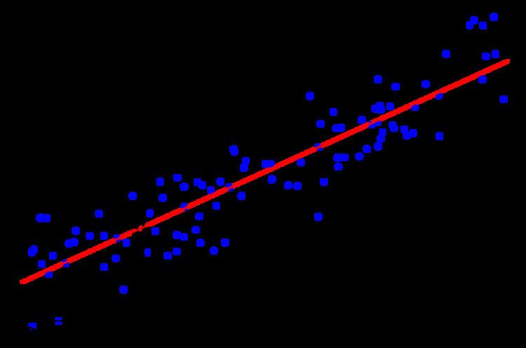
When only one dependent variable is being modeled, a scatterplot will suggest the form and strength of the relationship between the dependent variable and regressors. It might also reveal outliers, heteroscedasticity, and other aspects of the data that may complicate the interpretation of a fitted regression model. The scatterplot suggests that the relationship is strong and can be approximated as a quadratic function. OLS can handle non-linear relationships by introducing the regressor HEIGHT². The regression model then becomes a multiple linear model:

w i = β 1 + β 2 h i + β 3 h i 2 + ε i .

The output from most popular statistical packages will look similar to this:

In this table:

The Coefficient column gives the least squares estimates of parameters β_j

The Std errors column shows standard errors of each coefficient estimate: σ ^ j = ( σ ^ 2 [ Q x x − 1 ] j j ) 1 2

The t-statistic and p-value columns are testing whether any of the coefficients might be equal to zero. The t-statistic is calculated simply as t = β ^ j / σ ^ j . If the errors ε follow a normal distribution, t follows a Student-t distribution. Under weaker conditions, t is asymptotically normal. Large values of t indicate that the null hypothesis can be rejected and that the corresponding coefficient is not zero. The second column, p-value, expresses the results of the hypothesis test as a significance level. Conventionally, p-values smaller than 0.05 are taken as evidence that the population coefficient is nonzero.

R-squared is the coefficient of determination indicating goodness-of-fit of the regression. This statistic will be equal to one if fit is perfect, and to zero when regressors X have no explanatory power whatsoever. This is a biased estimate of the population R-squared, and will never decrease if additional regressors are added, even if they are irrelevant.

Adjusted R-squared is a slightly modified version of R 2 , designed to penalize for the excess number of regressors which do not add to the explanatory power of the regression. This statistic is always smaller than R 2 , can decrease as new regressors are added, and even be negative for poorly fitting models:

Log-likelihood is calculated under the assumption that errors follow normal distribution. Even though the assumption is not very reasonable, this statistic may still find its use in conducting LR tests.

Durbin–Watson statistic tests whether there is any evidence of serial correlation between the residuals. As a rule of thumb, the value smaller than 2 will be an evidence of positive correlation.

Akaike information criterion and Schwarz criterion are both used for model selection. Generally when comparing two alternative models, smaller values of one of these criteria will indicate a better model.

Standard error of regression is an estimate of σ, standard error of the error term.

Total sum of squares, model sum of squared, and residual sum of squares tell us how much of the initial variation in the sample were explained by the regression.

F-statistic tries to test the hypothesis that all coefficients (except the intercept) are equal to zero. This statistic has F(p–1,n–p) distribution under the null hypothesis and normality assumption, and its p-value indicates probability that the hypothesis is indeed true. Note that when errors are not normal this statistic becomes invalid, and other tests such as Wald test or LR test should be used.

Ordinary least squares analysis often includes the use of diagnostic plots designed to detect departures of the data from the assumed form of the model. These are some of the common diagnostic plots:

Residuals against the explanatory variables in the model. A non-linear relation between these variables suggests that the linearity of the conditional mean function may not hold. Different levels of variability in the residuals for different levels of the explanatory variables suggests possible heteroscedasticity.

Residuals against explanatory variables not in the model. Any relation of the residuals to these variables would suggest considering these variables for inclusion in the model.

Residuals against the fitted values, y ^ .

Residuals against the preceding residual. This plot may identify serial correlations in the residuals.

An important consideration when carrying out statistical inference using regression models is how the data were sampled. In this example, the data are averages rather than measurements on individual women. The fit of the model is very good, but this does not imply that the weight of an individual woman can be predicted with high accuracy based only on her height.

Sensitivity to rounding

This example also demonstrates that coefficients determined by these calculations are sensitive to how the data is prepared. The heights were originally given rounded to the nearest inch and have been converted and rounded to the nearest centimetre. Since the conversion factor is one inch to 2.54 cm this is not an exact conversion. The original inches can be recovered by Round(x/0.0254) and then re-converted to metric without rounding. If this is done the results become:

Using either of these equations to predict the weight of a 5' 6" (1.6764m) woman gives similar values: 62.94 kg with rounding vs. 62.98 kg without rounding. Thus a seemingly small variation in the data has a real effect on the coefficients but a small effect on the results of the equation.

While this may look innocuous in the middle of the data range it could become significant at the extremes or in the case where the fitted model is used to project outside the data range (extrapolation).

This highlights a common error: this example is an abuse of OLS which inherently requires that the errors in the independent variable (in this case height) are zero or at least negligible. The initial rounding to nearest inch plus any actual measurement errors constitute a finite and non-negligible error. As a result the fitted parameters are not the best estimates they are presumed to be. Though not totally spurious the error in the estimation will depend upon relative size of the x and y errors.