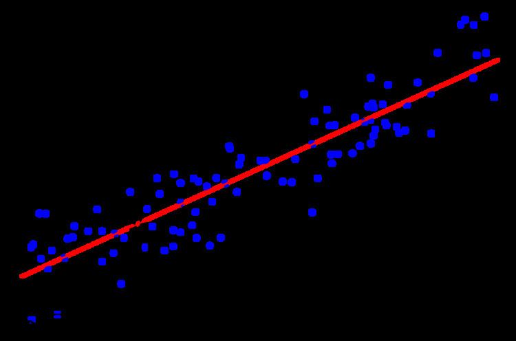
Quantile regression

Advantages and applications

Quantile regression is desired if conditional quantile functions are of interest. One advantage of quantile regression, relative to the ordinary least squares regression, is that the quantile regression estimates are more robust against outliers in the response measurements. However, the main attraction of quantile regression goes beyond that. Different measures of central tendency and statistical dispersion can be useful to obtain a more comprehensive analysis of the relationship between variables.

In ecology, quantile regression has been proposed and used as a way to discover more useful predictive relationships between variables in cases where there is no relationship or only a weak relationship between the means of such variables. The need for and success of quantile regression in ecology has been attributed to the complexity of interactions between different factors leading to data with unequal variation of one variable for different ranges of another variable.

Another application of quantile regression is in the areas of growth charts, where percentile curves are commonly used to screen for abnormal growth.

Quantile regression has also been applied to analyze hospital wait-times, where an analysis of extreme quantiles is of more interest than an analysis of the mean wait-time.

Mathematics

The mathematical forms arising from quantile regression are distinct from those arising in the method of least squares. The method of least squares leads to a consideration of problems in an inner product space, involving projection onto subspaces, and thus the problem of minimizing the squared errors can be reduced to a problem in numerical linear algebra. Quantile regression does not have this structure, and instead leads to problems in linear programming that can be solved by the simplex method.

History

The idea of estimating a median regression slope, a major theorem about minimizing sum of the absolute deviances and a geometrical algorithm for constructing median regression was proposed in 1760 by Ruđer Josip Bošković, a Jesuit Catholic priest from Dubrovnik. Median regression computations for larger data sets are quite tedious compared to the least squares method, for which reason it has historically generated a lack of popularity among statisticians, until the widespread adoption of computers in the latter part of the 20th century.

Quantiles

Let Y be a real valued random variable with cumulative distribution function F Y ( y ) = P ( Y ≤ y ) . The τ th quantile of Y is given by

Q Y ( τ ) = F Y − 1 ( τ ) = inf { y : F Y ( y ) ≥ τ }

where τ ∈ [ 0 , 1 ] .

Define the loss function as ρ τ ( y ) = y ( τ − I ( y < 0 ) ) , where I is an indicator function. A specific quantile can be found by minimizing the expected loss of Y − u with respect to u :

min u E ( ρ τ ( Y − u ) ) = min u ( τ − 1 ) ∫ − ∞ u ( y − u ) d F Y ( y ) + τ ∫ u ∞ ( y − u ) d F Y ( y ) .

This can be shown by setting the derivative of the expected loss function to 0 and letting q τ be the solution of

0 = ( 1 − τ ) ∫ − ∞ q τ d F Y ( y ) − τ ∫ q τ ∞ d F Y ( y ) .

This equation reduces to

0 = F Y ( q τ ) − τ ,

and then to

F Y ( q τ ) = τ .

Hence q τ is τ th quantile of the random variable Y.

Example

Let Y be a discrete random variable that takes values 1,2,..,9 with equal probabilities. The task is to find the median of Y, and hence the value τ = 0.5 is chosen. The expected loss, L(u), is

L ( u ) = ( τ − 1 ) 9 ∑ y i < u ( y i − u ) + τ 9 ∑ y i ≥ u ( y i − u ) = 0.5 9 ( − ∑ y i < u ( y i − u ) + ∑ y i ≥ u ( y i − u ) ) .

Since 0.5 / 9 is a constant, it can be taken out of the expected loss function (this is only true if τ = 0.5 ). Then, at u=3,

L ( 3 ) ∝ ∑ i = 1 2 − ( i − 3 ) + ∑ i = 3 9 ( i − 3 ) = [ ( 2 + 1 ) + ( 0 + 1 + 2 + . . . + 6 ) ] = 24.

Suppose that u is increased by 1 unit. Then the expected loss will be changed by ( 3 ) − ( 6 ) = − 3 on changing u to 4. If, u=5, the expected loss is

L ( 5 ) ∝ ∑ i = 1 4 i + ∑ i = 0 4 i = 20 ,

and any change in u will increase the expected loss. Thus u=5 is the median. The Table below shows the expected loss (divided by 0.5 / 9 ) for different values of u.

Intuition

Consider τ = 0.5 and let q be an initial guess for q τ . The expected loss evaluated at q is

− 0.5 ∫ − ∞ q ( y − q ) d F Y ( y ) + 0.5 ∫ q ∞ ( y − q ) d F Y ( y ) .

In order to minimize the expected loss, we move the value of q a little bit to see whether the expect loss will rise or fall. Suppose we increase q by 1 unit. Then the change of expected loss would be

∫ − ∞ q 1 d F Y ( y ) − ∫ q ∞ 1 d F Y ( y ) .

The first term of the equation is F Y ( q ) and second term of the equation is 1 − F Y ( q ) . Therefore the change of expected loss function is negative if and only if F Y ( q ) < 0.5 , that is if and only if q is smaller than the median. Similarly, if we reduce q by 1 unit, the change of expected loss function is negative if and only if q is larger than the median.

In order to minimize the expected loss function, we would increase (decrease) L(q) if q is smaller (larger) than the median, until q reaches the median. The idea behind the minimization is to count the number of points (weighted with the density) that are larger or smaller than q and then move q to a point where q is larger than τ % of the points.

Sample quantile

The τ sample quantile can be obtained by solving the following minimization problem

q ^ τ = arg min q ∈ R ∑ i = 1 n ρ τ ( y i − q ) , = arg min q ∈ R [ ( 1 − τ ) ∑ y i < q ( q − y i ) + τ ∑ y i ≥ q ( y i − q ) ] . The intuition is the same as for the population quantile.

Conditional quantile and quantile regression

Suppose the τ th conditional quantile function is Q Y | X ( τ ) = X β τ . Given the distribution function of Y , β τ can be obtained by solving

β τ = arg min β ∈ R k E ( ρ τ ( Y − X β ) ) .

Solving the sample analog gives the estimator of β .

β τ ^ = arg min β ∈ R k ∑ i = 1 n ( ρ τ ( Y i − X β ) ) .

Computation

The minimization problem can be reformulated as a linear programming problem

min β + , β − , u + , u − ∈ R 2 k × R + 2 n { τ 1 n ′ u + + ( 1 − τ ) 1 n ′ u − | X ( β + − β − ) + u + − u − = Y } ,

where

β j + = max ( β j , 0 ) ,    β j − = − min ( β j , 0 ) ,     u j + = max ( u j , 0 ) ,    u j − = − min ( u j , 0 ) .

Simplex methods or interior point methods can be applied to solve the linear programming problem.

Asymptotic properties

For τ ∈ ( 0 , 1 ) , under some regularity conditions, β ^ τ is asymptotically normal:

n ( β ^ τ − β τ ) → d N ( 0 , τ ( 1 − τ ) D − 1 Ω x D − 1 ) ,

where

D = E ( f Y ( X β ) X X ′ ) and Ω x = E ( X ′ X ) .

Direct estimation of the asymptotic variance-covariance matrix is not always satisfactory. Inference for quantile regression parameters can be made with the regression rank-score tests or with the bootstrap methods.

Equivariance

See invariant estimator for background on invariance or see equivariance.

Scale equivariance

For any a > 0 and τ ∈ [ 0 , 1 ]

β ^ ( τ ; a Y , X ) = a β ^ ( τ ; Y , X ) , β ^ ( τ ; − a Y , X ) = − a β ^ ( 1 − τ ; Y , X ) .

Shift equivariance

For any γ ∈ R k and τ ∈ [ 0 , 1 ]

β ^ ( τ ; Y + X γ , X ) = β ^ ( τ ; Y , X ) + γ .

Equivariance to reparameterization of design

Let A be any p × p nonsingular matrix and τ ∈ [ 0 , 1 ]

β ^ ( τ ; Y , X A ) = A − 1 β ^ ( τ ; Y , X ) .

Invariance to monotone transformations

If h is a nondecreasing function on 'R, the following invariance property applies:

h ( Q Y | X ( τ ) ) ≡ Q h ( Y ) | X ( τ ) .

Example (1):

Let Y = ln ⁡ ( W ) and Q Y | X ( τ ) = X β τ , then Q W | X ( τ ) = exp ⁡ ( X β τ ) . The mean regression does not have the same property since E ⁡ ( ln ⁡ ( Y ) ) ≠ ln ⁡ ( E ⁡ ( Y ) ) .

Bayesian methods for Quantile Regression

Because quantile regression does not normally assume a parametric likelihood for the conditional distributions of Y|X, the Bayesian methods work with a working likelihood. A convenient choice is the asymmetric Laplacian likelihood, because the mode of the resulting posterior under a flat prior is the usual quantile regression estimates. The posterior inference, however, must be interpreted with care. Yang and He showed that one can have asymptotically valid posterior inference if the working likelihood is chosen to be the empirical likelihood.

Censored Quantile Regression

If the response variable is subject to censoring, the conditional mean is not identifiable without additional distributional assumptions, but the conditional quantile is often identifiable. For recent work on censored quantile regression, see: Portnoy and Wang and Wang

Example (2):

Let Y c = max ( 0 , Y ) and Q Y | X = X β τ , then Q Y c | X ( τ ) = max ( 0 , X β τ ) . This is the censored quantile regression model: estimated values can be obtained without making any distributional assumptions, but at the cost of computational difficulty, some of which can be avoided by using a simple three step censored quantile regression procedure as an approximation.

For random censoring on the response variables, the censored quantile regression of Portnoy (2003) provides consistent estimates of all identifiable quantile functions based on reweighting each censored point appropriately.

Implementations

Numerous statistical software packages include implementations of quantile regression:

Matlab function quantreg

Eviews, since version 6.

gretl.

R offers several packages that implement quantile regression, most notably quantreg by Roger Koenker, but also gbm, quantregForest and qrnn

SAS through proc quantreg (ver. 9.2) and proc quantselect (ver. 9.3).

Stata, via the qreg command.

Vowpal Wabbit, via --loss_function quantile.

Statsmodels package for Python, via --QuantReg

Mathematica package QuantileRegression.m[1] hosted at the MathematicaForPrediction project at GitHub.