 | ||
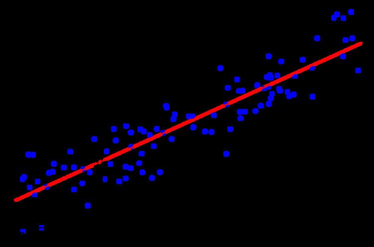
In statistics, generalized least squares (GLS) is a technique for estimating the unknown parameters in a linear regression model. GLS can be used to perform linear regression when there is a certain degree of correlation between the residuals in a regression model. In these cases, ordinary least squares and weighted least squares can be statistically inefficient, or even give misleading inferences. GLS was first described by Alexander Aitken in 1934.
Contents
Method outline
In a typical linear regression model we observe data
Here
Suppose
Since the objective is a quadratic form in
Properties
The GLS estimator is unbiased, consistent, efficient, and asymptotically normal:
GLS is equivalent to applying ordinary least squares to a linearly transformed version of the data. To see this, factor
This has the effect of standardizing the scale of the errors and “de-correlating” them. Since OLS is applied to data with homoscedastic errors, the Gauss–Markov theorem applies, and therefore the GLS estimate is the best linear unbiased estimator for β.
Weighted least squares
A special case of GLS called weighted least squares (WLS) occurs when all the off-diagonal entries of Ω are 0. This situation arises when the variances of the observed values are unequal (i.e. heteroscedasticity is present), but where no correlations exist among the observed variances. The weight for unit i is proportional to the reciprocal of the variance of the response for unit i.
Feasible generalized least squares
If the covariance of the errors
Whereas GLS is more efficient than OLS under heteroscedasticity or autocorrelation, this is not true for FGLS. The feasible estimator is, provided the errors covariance matrix is consistently estimated, asymptotically more efficient, but for a small or medium size sample, it can be actually less efficient than OLS. This is why, some authors prefer to use OLS, and reformulate their inferences by simply considering an alternative estimator for the variance of the estimator robust to heteroscedasticity or serial autocorrelation. But for large samples FGLS is preferred over OLS under heteroskedasticity or serial correlation. A cautionary note is that the FGLS estimator is not always consistent. One case in which FGLS might be inconsistent is if there are individual specific fixed effects.
In general this estimator has different properties than GLS. For large samples (i.e., asymptotically) all properties are (under appropriate conditions) common with respect to GLS, but for finite samples the properties of FGLS estimators are unknown: they vary dramatically with each particular model, and as a general rule their exact distributions cannot be derived analytically. For finite samples, FGLS may be even less efficient than OLS in some cases. Thus, while GLS can be made feasible, it is not always wise to apply this method when the sample is small. A method sometimes used to improve the accuracy of the estimators in finite samples is to iterate, i.e. taking the residuals from FGLS to update the errors covariance estimator, and then updating the FGLS estimation, applying the same idea iteratively until the estimators vary less than some tolerance. But this method does not necessarily improve the efficiency of the estimator very much if the original sample was small. A reasonable option when samples are not too large is to apply OLS, but throwing away the classical variance estimator
(which is inconsistent in this framework) and using a HAC (Heteroskedasticity and Autocorrelation Consistent) estimator. For example, in autocorrelation context we can use the Bartlett estimator (often known as Newey-West estimator since these authors popularized the use of this estimator among econometricians in their 1987 Econometrica article), and in heteroskedastic context we can use the Eicker–White estimator (Eicker–White). This approach is much safer, and it is the appropriate path to take unless the sample is large, and "large" is sometimes a slippery issue (e.g. if the errors distribution is asymmetric the required sample would be much larger).
The ordinary least squares (OLS) estimator is calculated as usual by
and estimates of the residuals
For simplicity consider the model for heteroskedastic errors. Assume that the variance-covariance matrix
It is important to notice that the squared residuals cannot be used in the previous expression; we need an estimator of the errors variances. To do so, we can use a parametric heteroskedasticity model, or a nonparametric estimator. Once this step is fulfilled, we can proceed:
Estimate
The procedure can be iterated. The first iteration is given by
This estimation of
Under regularity conditions any of the FGLS estimator (or that of any of its iterations, if we iterate a finite number of times) is asymptotically distributed as
where n is the sample size and
here p-lim means limit in probability
