Regularization (mathematics)

Introduction

In general, a regularization term R ( f ) is introduced to a general loss function:

min f ∑ i = 1 n V ( f ( x ^ i ) , y ^ i ) + λ R ( f )

for a loss function V that describes the cost of predicting f ( x ) when the label is y , such as the square loss or hinge loss, and for the term λ which controls the importance of the regularization term. R ( f ) is typically a penalty on the complexity of f , such as restrictions for smoothness or bounds on the vector space norm.

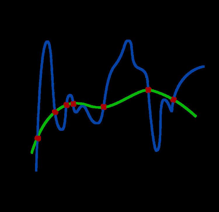
A theoretical justification for regularization is that it attempts to impose Occam's razor on the solution, as depicted in the figure. From a Bayesian point of view, many regularization techniques correspond to imposing certain prior distributions on model parameters.

Regularization can be used to learn simpler models, induce models to be sparse, introduce group structure into the learning problem, and more.

The same idea arose in many fields of science. For example, the least-squares method can be viewed as a very simple form of regularization. A simple form of regularization applied to integral equations, generally termed Tikhonov regularization after Andrey Nikolayevich Tikhonov, is essentially a trade-off between fitting the data and reducing a norm of the solution. More recently, non-linear regularization methods, including total variation regularization have become popular.

Generalization

Regularization can be motivated as a technique to improve the generalization of a learned model.

The goal of this learning problem is to find a function that fits or predicts the outcome (label) that minimizes the expected error over all possible inputs and labels. The expected error of a function f n is:

I [ f n ] = ∫ X × Y V ( f n ( x ) , y ) ρ ( x , y ) d x d y

Typically in learning problems, only a subset of input data and labels are available, measured with some noise. Therefore, the expected error is unmeasurable, and the best surrogate available is the empirical error over the N available samples:

I S [ f n ] = 1 n ∑ i = 1 N V ( f n ( x ^ i ) , y ^ i )

Without bounds on the complexity of the function space (formally, the reproducing kernel Hilbert space) available, a model will be learned that incurs zero loss on the surrogate empirical error. If measurements (e.g. of x i ) were made with noise, this model may suffer from overfitting and display poor expected error. Regularization introduces a penalty for exploring certain regions of the function space used to build the model, which can improve generalization.

Tikhonov regularization

When learning a linear function, such that f ( x ) = w ⋅ x , the L 2 norm loss corresponds to Tikhonov regularization. This is one of the most common forms of regularization, is also known as ridge regression, and is expressed as:

min w ∑ i = 1 n V ( x ^ i ⋅ w , y ^ i ) + λ ∥ w ∥ 2 2

In the case of a general function, we take the norm of the function in its reproducing kernel Hilbert space:

min f ∑ i = 1 n V ( f ( x ^ i ) , y ^ i ) + λ ∥ f ∥ H 2

As the L 2 norm is differentiable, learning problems using Tikhonov regularization can be solved by gradient descent.

Tikhonov regularized least squares

The learning problem with the least squares loss function and Tikhonov regularization can be solved analytically. Written in matrix form, the optimal w will be the one for which the gradient of the loss function with respect to w is 0.

min w 1 n ( X ^ w − Y ) T ( X ^ w − Y ) + λ ∥ w ∥ 2 2 ∇ w = 2 n X ^ T ( X ^ w − Y ) + 2 λ w       ← This is the first-order condition for this optimization problem 0 = X ^ T ( X ^ w − Y ) + n λ w w = ( X ^ T X ^ + λ n I ) − 1 ( X ^ T Y )

By construction of the optimization problem, other values of w would give larger values for the loss function. This could be verified by examining the second derivative ∇ w w .

During training, this algorithm takes O ( d 3 + n d 2 ) time. The terms correspond to the matrix inversion and calculating X T X , respectively. Testing takes O ( n d ) time.

Early stopping

Early stopping can be viewed as regularization in time. Intuitively, a training procedure like gradient descent will tend to learn more and more complex functions as the number of iterations increases. By regularizing on time, the complexity of the model can be controlled, improving generalization.

In practice, early stopping is implemented by training on a training set and measuring accuracy on a statistically independent validation set. The model is trained until performance on the validation set no longer improves. The model is then tested on a testing set.

Theoretical motivation in least squares

Consider the finite approximation of Neumann series for an invertible matrix A where ∥ I − A ∥ < 1 :

∑ i = 0 T − 1 ( I − A ) i ≈ A − 1

This can be used to approximate the analytical solution of unregularized least squares, if γ is introduced to ensure the norm is less than one.

w T = γ n ∑ i = 0 T − 1 ( I − γ n X ^ T X ^ ) i X ^ T Y ^

The exact solution to the unregularized least squares learning problem will minimize the empirical error, but may fail to generalize and minimize the expected error. By limiting T , the only free parameter in the algorithm above, the problem is regularized on time which may improve its generalization.

The algorithm above is equivalent to restricting the number of gradient descent iterations for the empirical risk

I s [ w ] = 1 2 n ∥ X ^ w − Y ^ ∥ R n 2

with the gradient descent update:

w 0 = 0 w t + 1 = ( I − γ n X ^ T X ^ ) w t + γ n X ^ T Y ^

The base case is trivial. The inductive case is proved as follows:

w T = ( I − γ n X ^ T X ^ ) γ n ∑ i = 0 T − 2 ( I − γ n X ^ T X ^ ) i X ^ T Y ^ + γ n X ^ T Y ^ w T = γ n ∑ i = 1 T − 1 ( I − γ n X ^ T X ^ ) i X ^ T Y ^ + γ n X ^ T Y ^ w T = γ n ∑ i = 0 T − 1 ( I − γ n X ^ T X ^ ) i X ^ T Y ^

Regularizers for sparsity

Assume that a dictionary ϕ j with dimension p is given such that a function in the function space can be expressed as:

f ( x ) = ∑ j = 1 p ϕ j ( x ) w j

Enforcing a sparsity constraint on w can lead to simpler and more interpretable models. This is useful in many real-life applications such as computational biology. An example is developing a simple predictive test for a disease in order to minimize the cost of performing medical tests while maximizing predictive power.

A sensible sparsity constraint is the L 0 norm ∥ w ∥ 0 , defined as the number of non-zero elements in w . Solving a L 0 regularized learning problem, however, has been demonstrated to be NP-hard.

The L 1 norm can be used to approximate the optimal L 0 norm via convex relaxation. It can be shown that the L 1 norm induces sparsity. In the case of least squares, this problem is known as LASSO in statistics and basis pursuit in signal processing.

min w ∈ R p 1 n ∥ X ^ w − Y ^ ∥ 2 + λ ∥ w ∥ 1

L 1 regularization can occasionally produce non-unique solutions. A simple example is provided in the figure when the space of possible solutions lies on a 45 degree line. This can be problematic for certain applications, and is overcome by combining L 1 with L 2 regularization in elastic net regularization, which takes the following form:

min w ∈ R p 1 n ∥ X ^ w − Y ^ ∥ 2 + λ ( α ∥ w ∥ 1 + ( 1 − α ) ∥ w ∥ 2 2 ) , α ∈ [ 0 , 1 ]

Elastic net regularization tends to have a grouping effect, where correlated input features are assigned equal weights.

Elastic net regularization is commonly used in practice and is implemented in many machine learning libraries.

Proximal methods

While the L 1 norm does not result in an NP-hard problem, it should be noted that the L 1 norm is convex but is not strictly diffentiable due to the kink at x = 0. Subgradient methods which rely on the subderivative can be used to solve L 1 regularized learning problems. However, faster convergence can be achieved through proximal methods.

For a problem min w ∈ H F ( w ) + R ( w ) such that F is convex, continuous, differentiable, with Lipschitz continuous gradient (such as the least squares loss function), and R is convex, continuous, and proper, then the proximal method to solve the problem is as follows. First define the proximal operator

prox R ⁡ ( v ) = argmin w ∈ R D ⁡ { R ( w ) + 1 2 ∥ w − v ∥ 2 } ,

and then iterate

w k + 1 = prox γ , R ⁡ ( w k − γ ∇ F ( w k ) )

The proximal method iteratively performs gradient descent and then projects the result back into the space permitted by R .

When R is the L 1 regularizer, the proximal operator is equivalent to the soft-thresholding operator,

S λ ( v ) f ( n ) = { v i − λ , if  v i > λ 0 , if  v i ∈ [ − λ , λ ] v i + λ , if  v i < − λ

This allows for efficient computation.

Group sparsity without overlaps

Groups of features can be regularized by a sparsity constraint, which can be useful for expressing certain prior knowledge into an optimization problem.

In the case of a linear model with non-overlapping known groups, a regularizer can be defined:

R ( w ) = ∑ g = 1 G ∥ w g ∥ g , where ∥ w g ∥ g = ∑ j = 1 | G g | ( w g j ) 2

This can be viewed as inducing a regularizer over the L 2 norm over members of each group followed by an L 1 norm over groups.

This can be solved by the proximal method, where the proximal operator is a block-wise soft-thresholding function:

( prox λ , R , g ⁡ ( w g ) ) j = { ( w g j − λ w g j ∥ w g ∥ g ) , if  ∥ w g ∥ g > λ 0 if  ∥ w g ∥ g ∈ [ − λ , λ ] ( w g j + λ w g j ∥ w g ∥ g ) , if  ∥ w g ∥ g < − λ

Group sparsity with overlaps

The algorithm described for group sparsity without overlaps can be applied to the case where groups do overlap, in certain situations. It should be noted that this will likely result in some groups with all zero elements, and other groups with some non-zero and some zero elements.

If it is desired to preserve the group structure, a new regularizer can be defined:

R ( w ) = inf { ∑ g = 1 G ∥ w g ∥ g : w = ∑ g = 1 G w ¯ g }

For each w g , w ¯ g is defined as the vector such that the restriction of w ¯ g to the group g equals w g and all other entries of w ¯ g are zero. The regularizer finds the optimal disintegration of w into parts. It can be viewed as duplicating all elements that exist in multiple groups. Learning problems with this regularizer can also be solved with the proximal method with a complication. The proximal operator cannot be computed in closed form, but can be effectively solved iteratively, inducing an inner iteration within the proximal method iteration.

Regularizers for semi-supervised learning

When labels are more expensive to gather than input examples, semi-supervised learning can be useful. Regularizers have been designed to guide learning algorithms to learn models that respect the structure of unsupervised training samples. If a symmetric weight matrix W is given, a regularizer can be defined:

R ( f ) = ∑ i , j w i j ( f ( x i ) − f ( x j ) ) 2

If W i j encodes the result of some distance metric for points x i and x j , it is desirable that f ( x i ) ≈ f ( x j ) . This regularizer captures this intuition, and is equivalent to:

R ( f ) = f ¯ T L f ¯ where L = D − W is the Laplacian matrix of the graph induced by W .

The optimization problem min f ∈ R m R ( f ) , m = u + l can be solved analytically if the constraint f ( x i ) = y i is applied for all supervised samples. The labeled part of the vector f is therefore obvious. The unlabeled part of f is solved for by:

min f u ∈ R u f T L f = min f u ∈ R u { f u T L u u f u + f l T L l u f u + f u T L u l f l } ∇ f u = 2 L u u f u + 2 L u l Y f u = L u u † ( L u l Y )

Note that the pseudo-inverse can be taken because L u l has the same range as L u u .

Regularizers for multitask learning

In the case of multitask learning, T problems are considered simultaneously, each related in some way. The goal is to learn T functions, ideally borrowing strength from the relatedness of tasks, that have predictive power. This is equivalent to learning the matrix W : T × D .

Sparse regularizer on columns

R ( w ) = ∑ i = 1 D ∥ W ∥ 2 , 1

This regularizer defines an L2 norm on each column and an L1 norm over all columns. It can be solved by proximal methods.

Nuclear norm regularization

R ( w ) = ∥ σ ( W ) ∥ 1 where σ ( W ) is the eigenvalues in the singular value decomposition of W .

Mean-constrained regularization

R ( f 1 ⋯ f T ) = ∑ t = 1 T ∥ f t − 1 T ∑ s = 1 T f s ∥ H k 2

This regularizer constrains the functions learned for each task to be similar to the overall average of the functions across all tasks. This is useful for expressing prior information that each task is expected to share similarities with each other task. An example is predicting blood iron levels measured at different times of the day, where each task represents a different person.

Clustered mean-constrained regularization

R ( f 1 ⋯ f T ) = ∑ r = 1 C ∑ t ∈ I ( r ) ∥ f t − 1 I ( r ) ∑ s ∈ I ( r ) f s ∥ H k 2 where I ( r ) is a cluster of tasks.

This regularizer is similar to the mean-constrained regularizer, but instead enforces similarity between tasks within the same cluster. This can capture more complex prior information. This technique has been used to predict Netflix recommendations. A cluster would correspond to a group of people who share similar preferences in movies.

Graph-based similarity

More general than above, similarity between tasks can be defined by a function. The regularizer encourages the model to learn similar functions for similar tasks.

R ( f 1 ⋯ f T ) = ∑ t , s = 1 , t ≠ s T ∥ f t − f s ∥ 2 M t s for a given symmetric similarity matrix M .

Other uses of regularization in statistics and machine learning

Bayesian learning methods make use of a prior probability that (usually) gives lower probability to more complex models. Well-known model selection techniques include the Akaike information criterion (AIC), minimum description length (MDL), and the Bayesian information criterion (BIC). Alternative methods of controlling overfitting not involving regularization include cross-validation.

Examples of applications of different methods of regularization to the linear model are: