
 | ||
In mathematics, the curve-shortening flow is a process that modifies a smooth curve in the Euclidean plane by moving its points perpendicularly to the curve at a speed proportional to the curvature. The curve-shortening flow is an example of a geometric flow, and is the one-dimensional case of the mean curvature flow. Other names for the same process include the Euclidean shortening flow, geometric heat flow, and arc length evolution.
Contents
- Definitions
- Non smooth curves
- Non Euclidean surfaces
- Space curves
- Beyond curves
- Avoidance principle radius and stretch factor
- Length
- Area
- Total absolute curvature
- GageHamiltonGrayson theorem
- Singularities of self crossing curves
- On Riemannian manifolds
- Huiskens monotonicity formula
- Curves with self similar evolution
- Ancient solutions
- Numerical approximations
- Front tracking
- Resampled convolution
- Median filtering
- Annealing metal sheets
- Shape analysis
- Reaction diffusion
- Cellular automata
- Construction of closed geodesics
- Related flows
- References
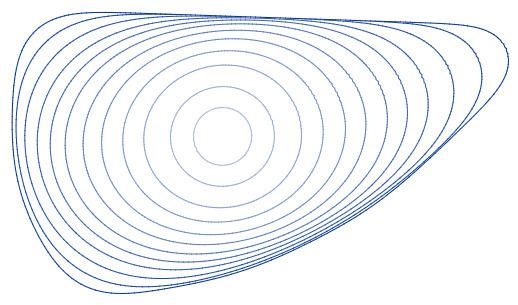
As the points of any smooth simple closed curve move in this way, the curve remains simple and smooth. It loses area at a constant rate, and its perimeter decreases as quickly as possible for any continuous curve evolution. If the curve is non-convex, its total absolute curvature decreases monotonically, until it becomes convex. Once convex, the isoperimetric ratio of the curve decreases as the curve converges to a circular shape, before collapsing to a single point of singularity. If two disjoint simple smooth closed curves evolve, they remain disjoint until one of them collapses to a point. The circle is the only simple closed curve that maintains its shape under the curve-shortening flow, but some curves that cross themselves or have infinite length keep their shape, including the grim reaper curve, an infinite curve that translates upwards, and spirals that rotate while remaining the same size and shape.
An approximation to the curve-shortening flow can be computed numerically, by approximating the curve as a polygon and using the finite difference method to calculate the motion of each polygon vertex. Alternative methods include computing a convolution of polygon vertices and then resampling vertices on the resulting curve, or repeatedly applying a median filter to a digital image whose black and white pixels represent the inside and outside of the curve.
The curve-shortening flow was originally studied as a model for annealing of metal sheets. Later, it was applied in image analysis to give a multi-scale representation of shapes. It can also model reaction–diffusion systems, and the behavior of cellular automata. In pure mathematics, the curve-shortening flow can be used to find closed geodesics on Riemannian manifolds, and as a model for the behavior of higher-dimensional flows.
Definitions
A flow is a process in which the points of a mathematical space continuously change their locations or properties over time. More specifically, in a one-dimensional geometric flow such as the curve-shortening flow, the points undergoing the flow belong to a curve, and what changes is the shape of the curve, its embedding into the Euclidean plane determined by the locations of each of its points. In the curve-shortening flow, each point of a curve moves in the direction of a normal vector to the curve, at a rate proportional to the curvature. For an evolving curve represented by a two-parameter function C(s,t) where s parameterizes the arc length along the curve and t parameterizes a time in the evolution of the curve, the curve-shortening flow can be described by the parabolic partial differential equation
a form of the heat equation, where κ is the curvature and n is the unit normal vector.
Because the ingredients of this equation, the arc length, curvature, and time, are all unaffected by translations and rotations of the Euclidean plane, it follows that the flow defined by this equation is invariant under translations and rotations (or more precisely, equivariant). If the plane is scaled by a constant dilation factor, the flow remains essentially unchanged, but is slowed down or sped up by the same factor.
Non-smooth curves
In order for the flow to be well defined, the given curve must be sufficiently smooth that it has a continuous curvature. However, once the flow starts, the curve becomes analytic, and remains so until reaching a singularity at which the curvature blows up. For a smooth curve without crossings, the only possible singularity happens when the curve collapses to a point, but immersed curves can have other types of singularity. In such cases, with some care it is possible to continue the flow past these singularities until the whole curve shrinks to a single point.
For a simple closed curve, using an extension of the flow to non-smooth curves based on the level set method, there are only two possibilities. Curves with zero Lebesgue measure (including all polygons and piecewise-smooth curves) instantly evolve into smooth curves, after which they evolve as any smooth curve would. However, Osgood curves with nonzero measure instead immediately evolve into a topological annulus with nonzero area and smooth boundaries. The topologist's sine curve is an example that instantly becomes smooth, despite not even being locally connected; examples such as this show that the reverse evolution of the curve-shortening flow can take well-behaved curves to complicated singularities in a finite amount of time.
Non-Euclidean surfaces
The curve-shortening flow, and many of the results about the curve-shortening flow, can be generalized from the Euclidean plane to any two-dimensional Riemannian manifold. In order to avoid additional types of singularity, it is important for the manifold to be convex at infinity; this is defined to mean that every compact set has a compact convex hull, as defined using geodesic convexity. The curve-shortening flow cannot cause a curve to depart from its convex hull, so this condition prevents parts of the curve from reaching the boundary of the manifold.
Space curves
The curve-shortening flow has also been studied for curves in three-dimensional Euclidean space. The normal vector in this case can be defined (as in the plane) as the derivative of the tangent vector with respect to arc length, normalized to be a unit vector; it is one of the components of the Frenet–Serret frame. It is not well defined at points of zero curvature, but the product of the curvature and the normal vector remains well defined at those points, allowing the curve-shortening flow to be defined. Curves in space may cross each other or themselves according to this flow, and the flow may lead to singularities in the curves; every singularity is asymptotic to a plane. The curve shortening flow for space curves has been used as a way to define flow past singularities in plane curves.
Beyond curves
It is possible to extend the definition of the flow to more general inputs than curves, for instance by using rectifiable varifolds or the level set method. However, these extended definitions may allow parts of curves to vanish instantaneously or fatten into sets of nonzero area.
A commonly studied variation of the problem involves networks of interior-disjoint smooth curves, with junctions where three or more of the curves meet. When the junctions all have exactly three curves meeting at angles of 2π/3 (the same conditions seen in an optimal Steiner tree or two-dimensional foam of soap bubbles) the flow is well-defined for the short term. However, it may eventually reach a singular state with four or more curves meeting at a junction, and there may be more than one way to continue the flow past such a singularity.
Avoidance principle, radius, and stretch factor
If two disjoint smooth simple closed curves undergo the curve-shortening flow simultaneously, they remain disjoint as the flow progresses. The reason is that, if two smooth curves move in a way that creates a crossing, then at the time of first crossing the curves would necessarily be tangent to each other, without crossing. But, in such a situation, the two curves' curvatures at the point of tangency would necessarily pull them apart rather than pushing them together into a crossing. For the same reason, a single simple closed curve can never evolve to cross itself. This phenomenon is known as the avoidance principle.
The avoidance principle implies that any smooth curve eventually either reaches a singularity (such as a point of infinite curvature) or collapses to a point. For, if a given smooth curve C is surrounded by a circle, both will remain disjoint until one or the other collapses or reaches a singularity. But the enclosing circle shrinks under the curvature flow, remaining circular, until it collapses, and by the avoidance principle C must remain contained within it. By the same reasoning, the radius of the smallest circle that encloses C must decrease at a rate that is at least as fast as the decrease in radius of a circle undergoing the same flow.
Huisken (1998) quantifies the avoidance principle for a single curve in terms of the ratio between the arc length (of the shorter of two arcs) and Euclidean distance between pairs of points, sometimes called the stretch factor. He shows that the stretch factor is strictly decreasing at each of its local maxima, except for the case of the two ends of a diameter of a circle in which case the stretch factor is constant at π. This monotonicity property implies the avoidance principle, for if the curve would ever touch itself the stretch factor would become infinite at the two touching points.
Length
As a curve undergoes the curve-shortening flow, its length L decreases at a rate given by the formula
where the interval is taken over the curve, κ is the curvature, and s is arc length along the curve. The integrand is always non-negative, and for any smooth closed curve there exist arcs within which it is strictly positive, so the length decreases monotonically. More generally, for any evolution of curves whose normal speed is f, the rate of change in length is
which can be interpreted as a negated inner product between the given evolution and the curve-shortening flow. Thus, the curve-shortening flow can be described as the gradient flow for length, the flow that (locally) decreases the length of the curve as quickly as possible relative to the L2 norm of the flow. This property is the one that gives the curve-shortening flow its name.
Area
For a simple closed curve, the area enclosed by the curve shrinks, at the constant rate of 2π units of area per unit of time, independent of the curve. Therefore, the total time for a curve to shrink to a point is proportional to its area, regardless of its initial shape. Because the area of a curve is reduced at a constant rate, and (by the isoperimetric inequality) a circle has the greatest possible area among simple closed curves of a given length, it follows that circles are the slowest curves to collapse to a point under the curve-shortening flow. All other curves take less time to collapse than a circle of the same length.
The constant rate of area reduction is the only conservation law satisfied by the curve-shortening flow. This implies that it is not possible to express the "vanishing point" where the curve eventually collapses as an integral over the curve of any function of its points and their derivatives, because such an expression would lead to a forbidden second conservation law. However, by combining the constant rate of area loss with the avoidance principle, it is possible to prove that the vanishing point always lies within a circle, concentric with the minimum enclosing circle, whose area is the difference in areas between the enclosing circle and the given curve.
Total absolute curvature
The total absolute curvature of a smooth curve is the integral of the absolute value of the curvature along the arc length of the curve,
It can also be expressed as a sum of the angles between the normal vectors at consecutive pairs of inflection points. It is 2π for convex curves and larger for non-convex curves, serving as a measure of non-convexity of a curve.
New inflection points cannot be created by the curve-shortening flow. Each of the angles in the representation of the total absolute curvature as a sum decreases monotonically, except at the instants when two consecutive inflection points reach the same angle or position as each other and are both eliminated. Therefore, the total absolute curvature can never increase as the curve evolves. For convex curves it is constant at 2π and for non-convex curves it decreases monotonically.
Gage–Hamilton–Grayson theorem
If a smooth simple closed curve undergoes the curve-shortening flow, it remains smoothly embedded without self-intersections. It will eventually become convex, and once it does so it will remain convex. After this time, all points of the curve will move inwards, and the shape of the curve will converge to a circle as the whole curve shrinks to a single point. This behavior is sometimes summarized by saying that every simple closed curve shrinks to a "round point".
This result is due to Michael Gage, Richard S. Hamilton, and Matthew Grayson. Gage (1983, 1984) proved convergence to a circle for convex curves that contract to a point. More specifically Gage showed that the isoperimetric ratio (the ratio of squared curve length to area, a number that is 4π for a circle and larger for any other convex curve) decreases monotonically and quickly. Gage & Hamilton (1986) proved that all smooth convex curves eventually contract to a point without forming any other singularities, and Grayson (1987) proved that every non-convex curve will eventually become convex. Andrews & Bryan (2011) provide a simpler proof of Grayson's result, based on the monotonicity of the stretch factor.
Similar results can be extended from closed curves to unbounded curves satisfying a local Lipschitz condition. For such curves, if both sides of the curve have infinite area, then the evolved curve remains smooth and singularity-free for all time. However, if one side of an unbounded curve has finite area, and the curve has finite total absolute curvature, then its evolution reaches a singularity in time proportional to the area on the finite-area side of the curve, with unbounded curvature near the singularity. For curves that are graphs of sufficiently well-behaved functions, asymptotic to a ray in each direction, the solution converges in shape to a unique shape that is asymptotic to the same rays. For networks formed by two disjoint rays on the same line, together with two smooth curves connecting the endpoints of the two rays, an analogue of the Gage–Hamilton–Grayson theorem holds, under which the region between the two curves becomes convex and then converges to a vesica piscis shape.
Singularities of self-crossing curves
Curves that have self-crossings may reach singularities before contracting to a point. For instance, if a lemniscate (any smooth immersed curve with a single crossing, resembling a figure 8 or infinity symbol) has unequal areas in its two lobes, then eventually the smaller lobe will collapse to a point. However, if the two lobes have equal areas, then they will remain equal throughout the evolution of the curve, and the isoperimetric ratio will diverge as the curve collapses to a singularity.
When a locally convex self-crossing curve approaches a singularity as one of its loops shrinks, it either shrinks in a self-similar way or asymptotically approaches the grim reaper curve (described below) as it shrinks. When a loop collapses to a singularity, the amount of total absolute curvature that is lost is either at least 2π or exactly π.
On Riemannian manifolds
On a Riemannian manifold, any smooth simple closed curve will remain smooth and simple as it evolves, just as in the Euclidean case. It will either collapse to a point in a finite amount of time, or remain smooth and simple forever. In the latter case, the curve necessarily converges to a closed geodesic of the surface.
Immersed curves on Riemannian manifolds, with finitely many self-crossings, become self-tangent only at a discrete set of times, at each of which they lose a crossing. As a consequence the number of self-crossing points is non-decreasing.
Huisken's monotonicity formula
According to Huisken's monotonicity formula, the convolution of an evolving curve with a time-reversed heat kernel is non-increasing. This result can be used to analyze the singularities of the evolution.
Curves with self-similar evolution
Because every other simple closed curve converges to a circle, the circle is the only simple closed curve that keeps its shape under the curve-shortening flow. However, there are many other examples of curves that are either non-simple (they include self-crossings) or non-closed (they extend to infinity) and keep their shape. In particular,
Ancient solutions
An ancient solution to a flow problem is a curve whose evolution can be extrapolated backwards for all time, without singularities. All of the self-similar solutions that shrink or stay the same size rather than growing are ancient solutions in this sense; they can be extrapolated backwards by reversing the self-similarity transformation that they would undergo by the forwards curve-shortening flow. Thus, for instance, the circle, grim reaper, and Abresch–Langer curves are all ancient solutions.
The only closed curves other than the circle and Abresch–Langer curves that form ancient solutions are a class of curves called the Angenent ovals after the work of Angenent (1992). These curves may be parameterized by specifying their curvature as a function of the tangent angle using the formula
and have as their limiting shape under reverse evolution a pair of grim reaper curves approaching each other from opposite directions. In the Cartesian coordinate system, they may be given by the implicit curve equation
In the physics literature, the same shapes are known as the paperclip model.
For more general classes of curves, such as the graphs of functions, a more diverse collection of ancient solutions is known.
Numerical approximations
In order to compute the curve-shortening flow efficiently, both a continuous curve and the continuous evolution of the curve need to be replaced by a discrete approximation.
Front tracking
Front tracking methods have long been used in fluid dynamics to model and track the motion of boundaries between different materials, of steep gradients in material properties such as weather fronts, or of shock waves within a single material. These methods involve deriving the equations of motion of the boundary, and using them to directly simulate the motion of the boundary, rather than simulating the underlying fluid and treating the boundary as an emergent property of the fluid. The same methods can also be used to simulate the curve-shortening flow, even when the curve undergoing the flow is not a boundary or shock.
In front tracking methods for curve shortening, the curve undergoing the evolution is discretized as a polygon. The finite difference method is used to derive formulas for the approximate normal vector and curvature at each vertex of the polygon, and these values are used to determine how to move each vertex in each time step. In some cases the normal motion of the points is combined with a tangential motion to spread them more uniformly around the curve. Merriman, Bence & Osher (1992) write that these methods are fast and accurate but that it is much more complicated to extend them to versions of the curve-shortening flow that apply to more complicated inputs than simple closed curves, where it is necessary to deal with singularities and changes of topology.
For most such methods, Cao (2003) warns that "The conditions of stability cannot be determined easily and the time step must be chosen ad hoc." Another finite differencing method by Crandall & Lions (1996) modifies the formula for the curvature at each vertex by adding to it a small term based on the Laplace operator. This modification is called elliptic regularization, and it can be used to help prove the existence of generalized flows as well as in their numerical simulation. Using it, the method of Crandall and Lions can be proven to converge and is the only numerical method listed by Cao that is equipped with bounds on its convergence rate. For an empirical comparison of the forward Euler, backward Euler, and more accurate Crank–Nicolson finite difference methods, see Balažovjech & Mikula (2009).
Resampled convolution
Mokhtarian & Mackworth (1992) suggest a numerical method for computing an approximation to the curve-shortening flow that maintains a discrete approximation to the curve and alternates between two steps:
As they show, this method converges to the curve-shortening distribution in the limit as the number of sample points grows and the normalized arc length of the convolution radius shrinks.
Median filtering
Merriman, Bence & Osher (1992) describe a scheme operating on a two-dimensonal square grid – effectively an array of pixels. The curve to be evolved is represented by assigning the value 0 (black) to pixels exterior to the curve, and 1 (white) to pixels interior to the curve, giving the indicator function for the interior of the curve. This representation is updated by alternating two steps:
In order for this scheme to be accurate, the time step must be large enough to cause the curve to move by at least one pixel even at points of low curvature, but small enough to cause the radius of blurring to be less than the minimum radius of curvature. Therefore, the size of a pixel must be O(min κ/max κ2), small enough to allow a suitable intermediate time step to be chosen.
The method can be generalized to the evolution of networks of curves, meeting at junctions and dividing the plane into more than three regions, by applying the same method simultaneously to each region. Instead of blurring and thresholding, this method can alternatively be described as applying a median filter with Gaussian weights to each pixel. It is possible to use kernels other than the heat kernel, or to adaptively refine the grid so that it has high resolution near the curve but does not waste time and memory on pixels far from the curve that do not contribute to the outcome. Instead of using only the two values in the pixelated image, a version of this method that uses an image whose pixel values represent the signed distance to the curve can achieve subpixel accuracy and require lower resolution.
Annealing metal sheets
An early reference to the curve-shortening flow by William W. Mullins (1956) motivates it as a model for the physical process of annealing, in which heat treatment causes the boundaries between grains of crystallized metal to shift. Unlike soap films, which are forced by differences in air pressure to become surfaces of constant mean curvature, the grain boundaries in annealing are subject only to local effects, which cause them to move according to the mean curvature flow. The one-dimensional case of this flow, the curve-shortening flow, corresponds to annealing sheets of metal that are thin enough for the grains to become effectively two-dimensional and their boundaries to become one-dimensional.
Shape analysis
In image processing and computer vision, Mokhtarian & Mackworth (1992) suggest applying the curve-shortening flow to the outline of a shape derived from a digital image, in order to remove noise from the shape and provide a scale space that provides a simplified description of the shape at different levels of resolution. The method of Mokhtarian and Mackworth involves computing the curve-shortening flow, tracking the inflection points of the curve as they progress through the flow, and drawing a graph that plots the positions of the inflection points around the curve against the time parameter. The inflection points will typically be removed from the curve in pairs as the curve becomes convex (according to the Gage–Hamilton–Grayson theorem) and the lifetime of a pair of points corresponds to the salience of a feature of the shape. Because of the resampled convolution method that they describe for computing a numerical approximation of the curve-shortening flow, they call their method the resampled curvature scale space. They observe that this scale space is invariant under Euclidean transformations of the given shape, and assert that it uniquely determines the shape and is robust against small variations in the shape. They compare it experimentally against several related alternative definitions of a scale space for shapes, and find that the resampled curvature scale space is less computationally intensive, more robust against nonuniform noise, and less strongly influenced by small-scale shape differences.
Reaction-diffusion
In reaction–diffusion systems modeled by the Allen–Cahn equation, the limiting behavior for fast reaction, slow diffusion, and two or more local minima of energy with the same energy level as each other is for the system to settle into regions of different local minima, with the fronts delimiting boundaries between these regions evolving according to the curve-shortening flow.
Cellular automata
In a cellular automaton, each cell in an infinite grid of cells may have one of a finite set of states, and all cells update their states simultaneously based only on the configuration of a small set of neighboring cells. A Life-like cellular automaton rule is one in which the grid is the infinite square lattice, there are exactly two cell states, the set of neighbors of each cell are the eight neighbors of the Moore neighborhood, and the update rule depends only on the number of neighbors with each of the two states rather than on any more complicated function of those states. In one particular life-like rule, introduced by Gerard Vichniac and called the twisted majority rule or annealing rule, the update rule sets the new value for each cell to be the majority among the nine cells given by it and its eight neighbors, except when these cells are split among four with one state and five with the other state, in which case the new value of the cell is the minority rather than the majority. The detailed dynamics of this rule are complicated, including the existence of small stable structures. However, in the aggregate (when started with all cells in random states) it tends to form large regions of cells that are all in the same state as each other, with the boundaries between these regions evolving according to the curve-shortening flow.
Construction of closed geodesics
The curve-shortening flow can be used to prove an isoperimetric inequality for surfaces whose Gaussian curvature is a non-increasing function of the distance from the origin, such as the paraboloid. On such a surface, the smooth compact set that has any given area and minimum perimeter for that area is necessarily a circle centered at the origin. The proof applies the curve-shortening flow to two curves, a metric circle and the boundary of any other compact set, and compares the change in perimeter of the two curves as they are both reduced to a point by the flow. The curve-shortening flow can also be used to prove the theorem of the three geodesics, that every smooth Riemannian manifold topologically equivalent to a sphere has three geodesics that form simple closed curves.
Related flows
Other geometric flows related to the curve-shortening flow include the following ones.