Backward Euler method

Description

Consider the ordinary differential equation

with initial value y ( t 0 ) = y 0 . Here the function f and the initial data t 0 and y 0 are known; the function y depends on the real variable t and is unknown. A numerical method produces a sequence y 0 , y 1 , y 2 , … such that y k approximates y ( t 0 + k h ) , where h is called the step size.

The backward Euler method computes the approximations using

This differs from the (forward) Euler method in that the latter uses f ( t k , y k ) in place of f ( t k + 1 , y k + 1 ) .

The backward Euler method is an implicit method: the new approximation y k + 1 appears on both sides of the equation, and thus the method needs to solve an algebraic equation for the unknown y k + 1 . Sometimes, this can be done by fixed-point iteration:

If this sequence converges (within a given tolerance), then the method takes its limit as the new approximation y k + 1 .

Alternatively, one can use (some modification of) the Newton–Raphson method to solve the algebraic equation.

Derivation

Integrating the differential equation d y d t = f ( t , y ) from t n to t n + 1 = t n + h yields

Now approximate the integral on the right by the right-hand rectangle method (with one rectangle):

Finally, use that y n is supposed to approximate y ( t n ) and the formula for the backward Euler method follows.

The same reasoning leads to the (standard) Euler method if the left-hand rectangle rule is used instead of the right-hand one.

Analysis

The backward Euler method has order one. This means that the local truncation error (defined as the error made in one step) is O ( h 2 ) , using the big O notation. The error at a specific time t is O ( h ) .

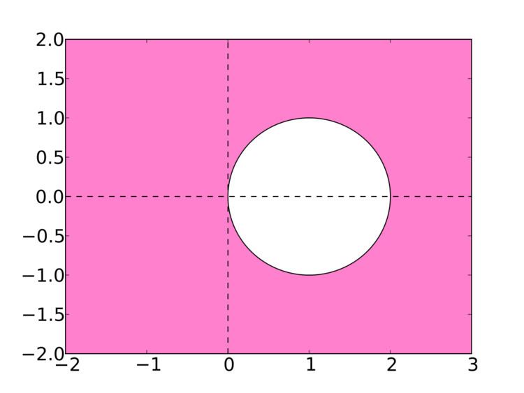
The region of absolute stability for the backward Euler method is the complement in the complex plane of the disk with radius 1 centered at 1, depicted in the figure. This includes the whole left half of the complex plane, so the backward Euler method is A-stable, making it suitable for the solution of stiff equations. In fact, the backward Euler method is even L-stable.

Extensions and modifications

The backward Euler method is a variant of the (forward) Euler method. Other variants are the semi-implicit Euler method and the exponential Euler method.

The backward Euler method can be seen as a Runge–Kutta method with one stage, described by the Butcher tableau:

The backward Euler method can also be seen as a linear multistep method with one step. It is the first method of the family of Adams–Moulton methods, and also of the family of backward differentiation formulas.