Implicit curve - Alchetron, The Free Social Encyclopedia

In mathematics an implicit curve is a plane curve which is defined by an equation

The graph of a function is usually described by an equation y = f ( x ) and is called an explicit representation. The third essential description of a curve is the parametric one: (x(t), y(t)), where the x- and y-coordinates of curve points are represented by two functions x ( t ) , y ( t ) dependent on a common parameter t . The change of representations is unusually simple only, when the explicit representation y = f ( x ) is given: y − f ( x ) = 0 (implicit), ( t , f ( t ) ) (parametric).

Examples of implicit curves:

a line: x + 2 y − 3 = 0 ,
a circle: x 2 + y 2 − 4 = 0 ,
the Semicubical parabola: x 3 − y 2 = 0 ,
Cassini ovals ( x 2 + y 2 ) 2 − 2 c 2 ( x 2 − y 2 ) − ( a 4 − c 4 ) = 0 (see picture),
sin ⁡ ( x + y ) − cos ⁡ ( x y ) + 1 = 0 (see picture).

The first four examples are algebraic curves, but the last one is not algebraic. The first three examples possess simple parametric representations, which is not true for the 4th and 5th example. Especially the 5th example shows the possible complicated geometric structure of an implicit curve.

The implicit function theorem describes conditions, under which an equation F ( x , y ) = 0 can be solved (theoretically) for x and/or y. But in general the solution may be not conducted. This theorem is the key for the computation of essential geometric features of the curve: tangents, normals, curvature (see below). In practice implicit curves have an essential drawback: their visualization is difficult (see below). But there are computer programs, enabling to display an implicit curve (see weblinks). Special properties of implicit curves make them essential tools in geometry and computer graphic (see below).

An implicit curve with an equation F ( x , y ) = 0 can be considered as the level curve of level 0 of the surface z = F ( x , y ) (see third picture).

Formulas

For the following formulas the implicit curve will be defined by an equation F ( x , y ) = 0 , where function F meets the needed mathematical requirements. The partial derivatives of F are F x , F y , F x x .

Tangent and normal vector

A curve point ( x 0 , y 0 ) is regular, if

( F x ( x 0 , y 0 ) , F y ( x 0 , y 0 ) ) ≠ ( 0 , 0 ) , otherwise the point is singular.

The equation of the tangent at a regular point ( x 0 , y 0 ) is

F x ( x 0 , y 0 ) ( x − x 0 ) + F y ( x 0 , y 0 ) ( y − y 0 ) = 0 , and

n ( x 0 , y 0 ) = ( F x ( x 0 , y 0 ) , F y ( x 0 , y 0 ) ) T is a normal vector.

Curvature

Due to clarity of the formulas the arguments ( x 0 , y 0 ) are omitted:

κ = − F y 2 F x x + 2 F x F y F x y − F x 2 F y y ( F x 2 + F y 2 ) 3 / 2 is

the curvature at a regular point..

Derivation of the formulas

The implicit function theorem guarantees within a neighborhood of a point ( x 0 , y 0 ) the existence of a function f such that F ( x , f ( x ) ) = 0 The derivatives of function f are (s. chain rule):

f ′ ( x ) = − F x ( x , f ( x ) ) F y ( x , f ( x ) )

f ″ = − F y 2 F x x + 2 F x F y F x y − F x 2 F y y F y 3 (The arguments were omitted.)

Inserting the derivatives of function f into the formulas for a tangent and curvature of the graph ( x , f ( x ) ) :

y = f ( x 0 ) + f ′ ( x 0 ) ( x − x 0 ) (tangent)

κ ( x 0 ) = f ″ ( x 0 ) ( 1 + f ′ ( x 0 ) 2 ) 3 / 2 (curvature)

one gets the formulas above

Disadvantage

The essential disadvantage of an implicit curve is the lack of an easy possibility to calculate single points which is necessary for visualization of an implicit curve (s. next section).

Advantages

Implicit representations facilitates the computation of intersection points: In case that one curve is represented implicitly and the other parametrically the computation of intersection points needs only a simple (1-dimensional) Newton iteration which is contrary to the cases implicit-implicit and parametric-parametric (see intersection).
An implicit representation F ( x , y ) = 0 gives the possibility to separate points not on the curve by the sign of F ( x , y ) . This may be helpful for example applying the false position method instead of a Newton iteration.
It is easy to generate curves which are geometrically similar to the given implicit curve F ( x , y ) = 0 . Add just a small number: F ( x , y ) − c = 0 (see section smooth approximations).

Applications of implicit curves

Within mathematics implicit curves play a prominent role as algebraic curves. Besides these classical field implicit curves are used for designing curves of desired geometrical shapes. Here are two examples.

Smooth approximation of convex polygons

A smooth approximation of a convex polygon can be achieved in the following way: Let g i ( x , y ) = a i x + b i y + c i = 0 , i = 1 , … , n be the equations of the lines containing the edges of the polygon such that for an inner point of the polygon g i is positive than the implicit curve

F ( x , y ) = g 1 ( x , y ) ⋯ g n ( x , y ) − c = 0

with suitable parameters c are smooth (differentiable) approximations of the polygon. For example, the curves

F ( x , y ) = ( x + 1 ) ( − x + 1 ) y ( − x − y + 2 ) ( x − y + 2 ) − c = 0 for c = 0.03 , … , 0.6

are smooth approximations of a polygon with 5 edges (s. picture)

Remark 1:

In case of two lines

F ( x , y ) = g 1 ( x , y ) g 2 ( x , y ) − c = 0

one gets

a pencil of parallel lines, if the given lines are parallel or the pencil of hyperbolas, which have the given lines as asymptotes.

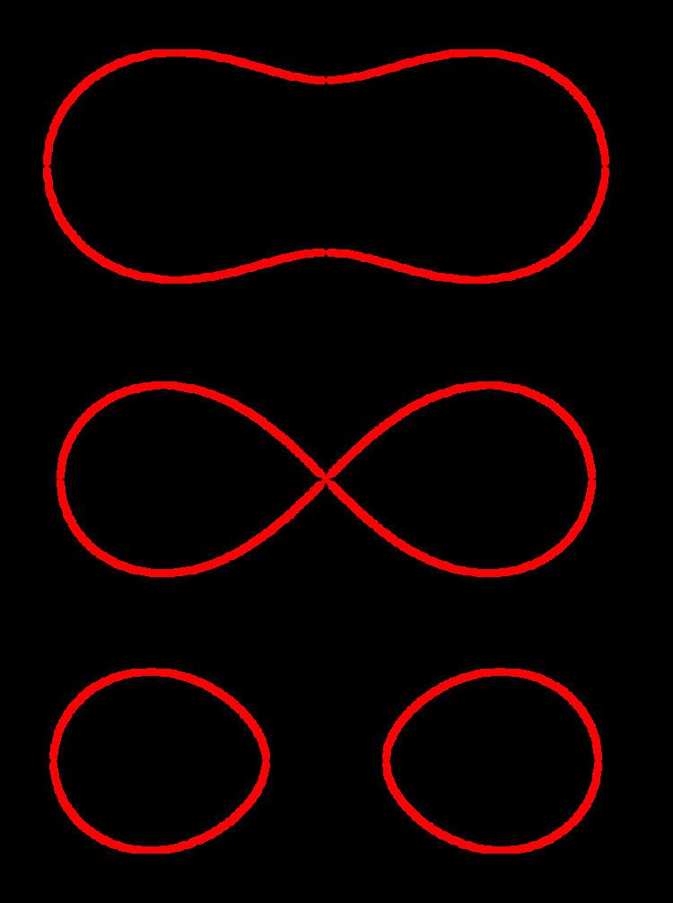
For example: The product of the coordinateaxes x y − c = 0 , c ≠ 0 , yields the pencil of hyperbolas, which have the coordinateaxes as asymptotes.

Remark 2:

If one starts with simple implicit curves other than lines (circles, parabolas,...) one gets a wide range of interesting new curves. For example

F ( x , y ) = y ( − x 2 − y 2 + 1 ) − c = 0

(product of a circle and the x-axis) yields smooth approximations of one half of a circle (s. picture) and

F ( x , y ) = ( − x 2 − ( y + 1 ) 2 + 4 ) ( − x 2 − ( y − 1 ) 2 + 4 ) − c = 0

(product of two circles) are smooth approximations of the intersection of two circles (s. picture).

Blending curves

In CAGD one uses implicit curves for the generation of blending curves, which are special curves establishing a smooth transition between two given curves. For example

F ( x , y ) = ( 1 − μ ) f 1 f 2 − μ ( g 1 g 2 ) 3 = 0

generates blending curves between the two circles

f 1 ( x , y ) = ( x − x 1 ) 2 + y 2 − r 1 2 = 0 , f 2 ( x , y ) = ( x − x 2 ) 2 + y 2 − r 2 2 = 0

The method guarantees the continuity of the tangents and curvatures at the points of contact. (s. picture). The two lines

g 1 ( x , y ) = x − x 1 = 0 , g 2 ( x , y ) = x − x 2 = 0

determine the points of contact at the circles. Parameter μ is a design parameter. For the picture: μ = 0.05 , … , 0.2 .

Visualization of an implicit curve

For visualizing an implicit curve one usually determines a polygon on the curve and displays the polygon. For a parametric curve this is an easy task: You just compute the points of a sequence of parametric values. For an implicit curve one has to solve two subproblems:

determination of a first curve point to a given starting point in the vicinity of the curve,
determination of a curve point starting from a known curve point.

In both cases it is reasonable to assume grad ⁡ F ≠ ( 0 , 0 ) . It seems a strong restriction. But in practice the assumption is not met in single points only.

Point algorithm

For the solution of both tasks mentioned above it is essential to have a computer program C P o i n t , which determines to a start point Q 0 = ( x 0 , y 0 ) in the vicinity of the curve a point P on the curve:

(P1) for the start point is j = 0 (P2) repeat ( x j + 1 , y j + 1 ) = ( x j , y j ) − F ( x j , y j ) F x ( x j , y j ) 2 + F y ( x j , y j ) 2 ( F x ( x j , y j ) , F y ( x j , y j ) ) ( Newton step for function g ( t ) = F ( x j + t F x ( x j , y j ) , y j + t F y ( x j , y j ) ) . ) (P3) until the distance between the points ( x j + 1 , y j + 1 ) , ( x j , y j ) is small enough. (P4) P = ( x j + 1 , y j + 1 ) is the curve point near the start point Q 0 .

Tracing algorithm

In order to generate a nearly equally spaced polygon on the implicit curve one chooses a step length s and

(T1) chooses a suitable starting point in the vicinity of the curve (T2) determines a first curve point P 1 using program C P o i n t (T3) determines the tangent (s. above), chooses a starting point on the tangent using step length s (s. picture) and determines a second curve point P 2 using program C P o i n t . ⋯

Because the algorithm traces the implicit curve it is called tracing algorithm. The algorithm traces only connected parts of the curve. If the implicit curve consists of several parts it has to be started several times with suitable starting points.

Raster algorithm

If the implicit curve consists of several or even unknown parts, the following raster algorithm is more convenient visualizing the curve:

(R1) Generate a net (raster) on the area of interest of the x-y-plane . (R2) choose any point of the raster as starting point for the point algorithm C P o i n t and mark the determined curvepoint.

If the net is dense enough one gets the impression of connected parts of the implicit curve. If for further applications polygons on the curves are needed one can trace parts of interest by the tracing algorithm.

Example: Given the implicit curve

F ( x , y ) = ( 3 x 2 − y 2 ) 2 y 2 − ( x 2 + y 2 ) 4 = 0

In order to demonstrate the algorithm the raster was widely spaced. The picture shows the single curve points determined by the raster algorithm. In order to accelerate the algorithm not every raster point was used as starting point.

Free Software

The following free software packages allow the visualization of implicit curves:

GeoGebra (algebraic curves only)

Gnuplot.

Additional software is mentioned in section Weblinks.

Implicit space curves

Any space curve which is defined by two equations

F ( x , y , z ) = 0 , G ( x , y , z ) = 0

is called implicit space curve.

A curve point ( x 0 , y 0 , z 0 ) is called regular,if the cross product of the gradients F and G is not ( 0 , 0 , 0 ) at this point:

t ( x 0 , y 0 , z 0 ) = grad ⁡ F ( x 0 , y 0 , z 0 ) × grad ⁡ G ( x 0 , y 0 , z 0 ) ≠ ( 0 , 0 , 0 )

otherwise singular. Vector t ( x 0 , y 0 , z 0 ) is a tangent vector of the curve at point ( x 0 , y 0 , z 0 ) .

Examples:

( 1 ) x + y + z − 1 = 0 , x − y + z − 2 = 0

( 2 ) x 2 + y 2 + z 2 − 4 = 0 , x + y + z − 1 = 0

( 3 ) x 2 + y 2 − 1 = 0 , x + y + z − 1 = 0

( 4 ) x 2 + y 2 + z 2 − 16 = 0 , ( y − y 0 ) 2 + z 2 − 9 = 0

For the computation of curve points and the visualizition of an implicit space curve see intersection.

References

Implicit curve Wikipedia

(Text) CC BY-SA

Contents