Finite difference method

Derivation from Taylor's polynomial

First, assuming the function whose derivatives are to be approximated is properly-behaved, by Taylor's theorem, we can create a Taylor Series expansion

f ( x 0 + h ) = f ( x 0 ) + f ′ ( x 0 ) 1 ! h + f ( 2 ) ( x 0 ) 2 ! h 2 + ⋯ + f ( n ) ( x 0 ) n ! h n + R n ( x ) ,

where n! denotes the factorial of n, and R_n(x) is a remainder term, denoting the difference between the Taylor polynomial of degree n and the original function. We will derive an approximation for the first derivative of the function "f" by first truncating the Taylor polynomial:

f ( x 0 + h ) = f ( x 0 ) + f ′ ( x 0 ) h + R 1 ( x ) ,

Setting, x₀=a we have,

f ( a + h ) = f ( a ) + f ′ ( a ) h + R 1 ( x ) ,

Dividing across by h gives:

f ( a + h ) h = f ( a ) h + f ′ ( a ) + R 1 ( x ) h

Solving for f'(a):

f ′ ( a ) = f ( a + h ) − f ( a ) h − R 1 ( x ) h

Assuming that R 1 ( x ) is sufficiently small, the approximation of the first derivative of "f" is:

f ′ ( a ) ≈ f ( a + h ) − f ( a ) h .

Accuracy and order

The error in a method's solution is defined as the difference between the approximation and the exact analytical solution. The two sources of error in finite difference methods are round-off error, the loss of precision due to computer rounding of decimal quantities, and truncation error or discretization error, the difference between the exact solution of the original differential equation and the exact quantity assuming perfect arithmetic (that is, assuming no round-off).

To use a finite difference method to approximate the solution to a problem, one must first discretize the problem's domain. This is usually done by dividing the domain into a uniform grid (see image to the right). Note that this means that finite-difference methods produce sets of discrete numerical approximations to the derivative, often in a "time-stepping" manner.

An expression of general interest is the local truncation error of a method. Typically expressed using Big-O notation, local truncation error refers to the error from a single application of a method. That is, it is the quantity f ′ ( x i ) − f i ′ if f ′ ( x i ) refers to the exact value and f i ′ to the numerical approximation. The remainder term of a Taylor polynomial is convenient for analyzing the local truncation error. Using the Lagrange form of the remainder from the Taylor polynomial for f ( x 0 + h ) , which is

R n ( x 0 + h ) = f ( n + 1 ) ( ξ ) ( n + 1 ) ! ( h ) n + 1 , where x 0 < ξ < x 0 + h ,

the dominant term of the local truncation error can be discovered. For example, again using the forward-difference formula for the first derivative, knowing that f ( x i ) = f ( x 0 + i h ) ,

f ( x 0 + i h ) = f ( x 0 ) + f ′ ( x 0 ) i h + f ″ ( ξ ) 2 ! ( i h ) 2 ,

and with some algebraic manipulation, this leads to

f ( x 0 + i h ) − f ( x 0 ) i h = f ′ ( x 0 ) + f ″ ( ξ ) 2 ! i h ,

and further noting that the quantity on the left is the approximation from the finite difference method and that the quantity on the right is the exact quantity of interest plus a remainder, clearly that remainder is the local truncation error. A final expression of this example and its order is:

f ( x 0 + i h ) − f ( x 0 ) i h = f ′ ( x 0 ) + O ( h ) .

This means that, in this case, the local truncation error is proportional to the step sizes. The quality and duration of simulated FDM solution depends on the discretization equation selection and the step sizes (time and space steps). The data quality and simulation duration increase significantly with smaller step size. Therefore, a reasonable balance between data quality and simulation duration is necessary for practical usage. Large time steps are useful for increasing simulation speed in practice. However, time steps which are too large may create instabilities and affect the data quality.

The von Neumann method is usually applied to determine the numerical model stability.

Example: ordinary differential equation

For example, consider the ordinary differential equation

u ′ ( x ) = 3 u ( x ) + 2.

The Euler method for solving this equation uses the finite difference quotient

u ( x + h ) − u ( x ) h ≈ u ′ ( x )

to approximate the differential equation by first substituting it for u'(x) then applying a little algebra (multiplying both sides by h, and then adding u(x) to both sides) to get

u ( x + h ) = u ( x ) + h ( 3 u ( x ) + 2 ) .

The last equation is a finite-difference equation, and solving this equation gives an approximate solution to the differential equation.

Example: The heat equation

Consider the normalized heat equation in one dimension, with homogeneous Dirichlet boundary conditions

U t = U x x U ( 0 , t ) = U ( 1 , t ) = 0 (boundary condition) U ( x , 0 ) = U 0 ( x ) (initial condition)

One way to numerically solve this equation is to approximate all the derivatives by finite differences. We partition the domain in space using a mesh x 0 , . . . , x J and in time using a mesh t 0 , . . . . , t N . We assume a uniform partition both in space and in time, so the difference between two consecutive space points will be h and between two consecutive time points will be k. The points

u ( x j , t n ) = u j n

will represent the numerical approximation of u ( x j , t n ) .

Explicit method

Using a forward difference at time t n and a second-order central difference for the space derivative at position x j (FTCS) we get the recurrence equation:

u j n + 1 − u j n k = u j + 1 n − 2 u j n + u j − 1 n h 2 .

This is an explicit method for solving the one-dimensional heat equation.

We can obtain u j n + 1 from the other values this way:

u j n + 1 = ( 1 − 2 r ) u j n + r u j − 1 n + r u j + 1 n

where r = k / h 2 .

So, with this recurrence relation, and knowing the values at time n, one can obtain the corresponding values at time n+1. u 0 n and u J n must be replaced by the boundary conditions, in this example they are both 0.

This explicit method is known to be numerically stable and convergent whenever r ≤ 1 / 2 . The numerical errors are proportional to the time step and the square of the space step:

Δ u = O ( k ) + O ( h 2 )

Implicit method

If we use the backward difference at time t n + 1 and a second-order central difference for the space derivative at position x j (The Backward Time, Centered Space Method "BTCS") we get the recurrence equation:

u j n + 1 − u j n k = u j + 1 n + 1 − 2 u j n + 1 + u j − 1 n + 1 h 2 .

This is an implicit method for solving the one-dimensional heat equation.

We can obtain u j n from solving a system of linear equations:

( 1 + 2 r ) u j n + 1 − r u j − 1 n + 1 − r u j + 1 n + 1 = u j n

The scheme is always numerically stable and convergent but usually more numerically intensive than the explicit method as it requires solving a system of numerical equations on each time step. The errors are linear over the time step and quadratic over the space step:

Δ u = O ( k ) + O ( h 2 ) .

Crank–Nicolson method

Finally if we use the central difference at time t n + 1 / 2 and a second-order central difference for the space derivative at position x j ("CTCS") we get the recurrence equation:

u j n + 1 − u j n k = 1 2 ( u j + 1 n + 1 − 2 u j n + 1 + u j − 1 n + 1 h 2 + u j + 1 n − 2 u j n + u j − 1 n h 2 ) .

This formula is known as the Crank–Nicolson method.

We can obtain u j n + 1 from solving a system of linear equations:

( 2 + 2 r ) u j n + 1 − r u j − 1 n + 1 − r u j + 1 n + 1 = ( 2 − 2 r ) u j n + r u j − 1 n + r u j + 1 n

The scheme is always numerically stable and convergent but usually more numerically intensive as it requires solving a system of numerical equations on each time step. The errors are quadratic over both the time step and the space step:

Δ u = O ( k 2 ) + O ( h 2 ) .

Usually the Crank–Nicolson scheme is the most accurate scheme for small time steps. The explicit scheme is the least accurate and can be unstable, but is also the easiest to implement and the least numerically intensive. The implicit scheme works the best for large time steps.

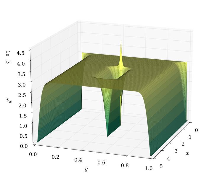
Comparison

The figures below present the solutions given by the above methods to approximate the heat equation

U t = α U x x , α = 1 π 2 ,

with the boundary condition

U ( 0 , t ) = U ( 1 , t ) = 0.

The exact solution is

U ( x , t ) = 1 π 2 e − t sin ⁡ ( π x ) .