Gaussian function

Properties

Gaussian functions arise by composing the exponential function with a concave quadratic function. The Gaussian functions are thus those functions whose logarithm is a concave quadratic function.

The parameter c is related to the full width at half maximum (FWHM) of the peak according to

The function may then be expressed in terms of the FWHM, represented by w:

Alternatively, the parameter c can be interpreted by saying that the two inflection points of the function occur at x = b − c and x = b + c.

The full width at tenth of maximum (FWTM) for a Gaussian could be of interest and is

Gaussian functions are analytic, and their limit as x → ∞ is 0 (for the above case of b = 0).

Gaussian functions are among those functions that are elementary but lack elementary antiderivatives; the integral of the Gaussian function is the error function. Nonetheless their improper integrals over the whole real line can be evaluated exactly, using the Gaussian integral

and one obtains

This integral is 1 if and only if a = 1 c 2 π , and in this case the Gaussian is the probability density function of a normally distributed random variable with expected value μ = b and variance σ² = c²:

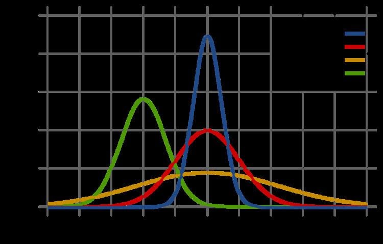
These Gaussians are plotted in the accompanying figure.

Gaussian functions centered at zero minimize the Fourier uncertainty principle.

The product of two Gaussian functions is a Gaussian, and the convolution of two Gaussian functions is also a Gaussian, with variance being the sum of the original variances: c 2 = c 1 2 + c 2 2 . The product of two Gaussian probability density functions, though, is not in general a Gaussian PDF.

Taking the Fourier transform (unitary, angular frequency convention) of a Gaussian function with parameters a = 1, b = 0 and c yields another Gaussian function, with parameters c , b = 0 and 1 c . So in particular the Gaussian functions with b = 0 and c = 1 are kept fixed by the Fourier transform (they are eigenfunctions of the Fourier transform with eigenvalue 1). A physical realization is that of the diffraction pattern: for example, a photographic slide whose transmittance has a Gaussian variation is also a Gaussian function.

The fact that the Gaussian function is an eigenfunction of the continuous Fourier transform allows us to derive the following interesting identity from the Poisson summation formula:

Integral of a Gaussian function

The integral of an arbitrary Gaussian function is

An alternative form is

where f must be strictly positive for the integral to converge.

Proof

The integral

for some real constants a, b, c > 0 can be calculated by putting it into the form of a Gaussian integral. First, the constant a can simply be factored out of the integral. Next, the variable of integration is changed from x to y = x - b.

and then to z = y / 2 c 2

Then, using the Gaussian integral identity

we have

Two-dimensional Gaussian function

In two dimensions, the power to which e is raised in the Gaussian function is any negative-definite quadratic form. Consequently, the level sets of the Gaussian will always be ellipses.

A particular example of a two-dimensional Gaussian function is

Here the coefficient A is the amplitude, x_o,y_o is the center and σ_x, σ_y are the x and y spreads of the blob. The figure on the right was created using A = 1, x_o = 0, y_o = 0, σ_x = σ_y = 1.

The volume under the Gaussian function is given by

In general, a two-dimensional elliptical Gaussian function is expressed as

where the matrix

is positive-definite.

Using this formulation, the figure on the right can be created using A = 1, (x_o, y_o) = (0, 0), a = c = 1/2, b = 0.

Meaning of parameters for the general equation

For the general form of the equation the coefficient A is the height of the peak and (x_o, y_o) is the center of the blob.

If we set

then we rotate the blob by a clockwise angle θ (for counterclockwise rotation invert the signs in the b coefficient). This can be seen in the following examples:

Using the following Octave code one can easily see the effect of changing the parameters

Such functions are often used in image processing and in computational models of visual system function—see the articles on scale space and affine shn.

Also see multivariate normal distribution.

Higher-order Gaussian or Super-Gaussian function

A more general formulation of a Gaussian function with a flat-top and Gaussian fall-off can be taken by raising the content of the exponent to a power, P :

f ( x ) = A exp ⁡ ( − ( ( x − x o ) 2 2 σ x 2 ) P ) . This function is known as a super-Gaussian function and is often used for Gaussian beam formulation. In a two-dimensional formulation, a Gaussian function along x and y can be combined with potentially different P x and P y to form an elliptical Gaussian distribution, f ( x , y ) = A exp ⁡ ( − ( ( x − x o ) 2 2 σ x 2 + ( y − y o ) 2 2 σ y 2 ) P ) or a rectangular Gaussian distribution, f ( x , y ) = A exp ⁡ ( − ( ( x − x o ) 2 2 σ x 2 ) P x − ( ( y − y o ) 2 2 σ y 2 ) P y ) .

Multi-dimensional Gaussian function

In an n -dimensional space a Gaussian function can be defined as

where x = { x 1 , … , x n } is a column of n coordinates, A is a positive-definite n × n matrix, and T denotes matrix transposition.

The integral of this Gaussian function over the whole n -dimensional space is given as

It can be easily calculated by diagonalizing the matrix A and changing the integration variables to the eigenvectors of A .

More generally a shifted Gaussian function is defined as

where s = { s 1 , … , s n } is the shift vector and the matrix A can be assumed to be symmetric, A T = A , and positive-definite. The following integrals with this function can be calculated with the same technique,

Gaussian profile estimation

A number of fields such as stellar photometry, Gaussian beam characterization, and emission/absorption line spectroscopy work with sampled Gaussian functions and need to accurately estimate the height, position, and width parameters of the function. These are a , b , and c for a 1D Gaussian function, A , ( x 0 , y 0 ) , and ( σ x , σ y ) for a 2D Gaussian function. The most common method for estimating the profile parameters is to take the logarithm of the data and fit a parabola to the resulting data set. While this provides a simple least squares fitting procedure, the resulting algorithm is biased by excessively weighting small data values, and this can produce large errors in the profile estimate. One can partially compensate for this through weighted least squares estimation, in which the small data values are given small weights, but this too can be biased by allowing the tail of the Gaussian to dominate the fit. In order to remove the bias, one can instead use an iterative procedure in which the weights are updated at each iteration (see Iteratively reweighted least squares).

Once one has an algorithm for estimating the Gaussian function parameters, it is also important to know how accurate those estimates are. While an estimation algorithm can provide numerical estimates for the variance of each parameter (i.e. the variance of the estimated height, position, and width of the function), one can use Cramér–Rao bound theory to obtain an analytical expression for the lower bound on the parameter variances, given some assumptions about the data.

1. The noise in the measured profile is either i.i.d. Gaussian, or the noise is Poisson-distributed.
2. The spacing between each sampling (i.e. the distance between pixels measuring the data) is uniform.
3. The peak is "well-sampled", so that less than 10% of the area or volume under the peak (area if a 1D Gaussian, volume if a 2D Gaussian) lies outside the measurement region.
4. The width of the peak is much larger than the distance between sample locations (i.e. the detector pixels must be at least 5 times smaller than the Gaussian FWHM).

When these assumptions are satisfied, the following covariance matrix K applies for the 1D profile parameters a , b , and c under i.i.d. Gaussian noise and under Poisson noise:

where δ x is the width of the pixels used to sample the function, Q is the quantum efficiency of the detector, and σ indicates the standard deviation of the measurement noise. Thus, the individual variances for the parameters are, in the Gaussian noise case,

and in the Poisson noise case,

For the 2D profile parameters giving the amplitude A , position ( x 0 , y 0 ) , and width ( σ x , σ y ) of the profile, the following covariance matrices apply:

where the individual parameter variances are given by the diagonal elements of the covariance matrix.

Discrete Gaussian

One may ask for a discrete analog to the Gaussian; this is necessary in discrete applications, particularly digital signal processing. A simple answer is to sample the continuous Gaussian, yielding the sampled Gaussian kernel. However, this discrete function does not have the discrete analogs of the properties of the continuous function, and can lead to undesired effects, as described in the article scale space implementation.

An alternative approach is to use discrete Gaussian kernel:

where I n ( t ) denotes the modified Bessel functions of integer order.

This is the discrete analog of the continuous Gaussian in that it is the solution to the discrete diffusion equation (discrete space, continuous time), just as the continuous Gaussian is the solution to the continuous diffusion equation.

Applications

Gaussian functions appear in many contexts in the natural sciences, the social sciences, mathematics, and engineering. Some examples include: