Cauchy–Riemann equations

Simple example

Suppose that z = x + iy. A complex-valued function f(z) = z² is differentiable at any point z in the complex plane.

f ( z ) = ( x + i y ) 2 = x 2 − y 2 + 2 i x y

The real part u(x, y) and the imaginary part v(x, y) of f(z) are

u ( x , y ) = x 2 − y 2 v ( x , y ) = 2 x y

respectively. The partial derivatives of these are

∂ u ∂ x = 2 x ∂ u ∂ y = − 2 y ∂ v ∂ x = 2 y ∂ v ∂ y = 2 x .

These partial derivatives have following relationships:

∂ u ∂ x = ∂ v ∂ y ∂ u ∂ y = − ∂ v ∂ x .

Thus this complex-valued function f(z) satisfies the Cauchy–Riemann equations.

( 1 a ) ∂ u ∂ x = ∂ v ∂ y ( 1 b ) ∂ u ∂ y = − ∂ v ∂ x

Interpretation and reformulation

The equations are one way of looking at the condition on a function to be differentiable in the sense of complex analysis: in other words they encapsulate the notion of function of a complex variable by means of conventional differential calculus. In the theory there are several other major ways of looking at this notion, and the translation of the condition into other language is often needed.

Conformal mappings

First, the Cauchy–Riemann equations may be written in complex form

(2)     i ∂ f ∂ x = ∂ f ∂ y .

In this form, the equations correspond structurally to the condition that the Jacobian matrix is of the form

( a − b b a ) ,

where a = ∂ u / ∂ x = ∂ v / ∂ y and b = ∂ v / ∂ x = − ∂ u / ∂ y . A matrix of this form is the matrix representation of a complex number. Geometrically, such a matrix is always the composition of a rotation with a scaling, and in particular preserves angles. The Jacobian of a function f(z) takes infinitesimal line segments at the intersection of two curves in z and rotates them to the corresponding segments in f(z). Consequently, a function satisfying the Cauchy–Riemann equations, with a nonzero derivative, preserves the angle between curves in the plane. That is, the Cauchy–Riemann equations are the conditions for a function to be conformal.

Moreover, because the composition of a conformal transformation with another conformal transformation is also conformal, the composition of a solution of the Cauchy–Riemann equations with a conformal map must itself solve the Cauchy–Riemann equations. Thus the Cauchy–Riemann equations are conformally invariant.

Complex differentiability

Suppose that

f ( z ) = u ( z ) + i ⋅ v ( z )

is a function of a complex number z. Then the complex derivative of f at a point z₀ is defined by

lim h → 0 h ∈ C f ( z 0 + h ) − f ( z 0 ) h = f ′ ( z 0 )

provided this limit exists.

If this limit exists, then it may be computed by taking the limit as h → 0 along the real axis or imaginary axis; in either case it should give the same result. Approaching along the real axis, one finds

lim h → 0 h ∈ R f ( z 0 + h ) − f ( z 0 ) h = ∂ f ∂ x ( z 0 ) .

On the other hand, approaching along the imaginary axis,

lim h → 0 h ∈ R f ( z 0 + i h ) − f ( z 0 ) i h = 1 i ∂ f ∂ y ( z 0 ) .

The equality of the derivative of f taken along the two axis is

i ∂ f ∂ x ( z 0 ) = ∂ f ∂ y ( z 0 ) ,

which are the Cauchy–Riemann equations (2) at the point z₀.

Conversely, if f : C → C is a function which is differentiable when regarded as a function on R², then f is complex differentiable if and only if the Cauchy–Riemann equations hold. In other words, if u and v are real-differentiable functions of two real variables, obviously u + iv is a (complex-valued) real-differentiable function, but u + iv is complex-differentiable if and only if the Cauchy–Riemann equations hold.

Indeed, following Rudin (1966), suppose f is a complex function defined in an open set Ω ⊂ C. Then, writing z = x + iy for every z ∈ Ω, one can also regard Ω as an open subset of R², and f as a function of two real variables x and y, which maps Ω ⊂ R² to C. We consider the Cauchy–Riemann equations at z = z₀. So assume f is differentiable at z₀, as a function of two real variables from Ω to C. This is equivalent to the existence of the following linear approximation

f ( z 0 + Δ z ) − f ( z 0 ) = f x Δ x + f y Δ y + η ( Δ z ) Δ z

where z = x + iy and η(Δz) → 0 as Δz → 0. Since Δ z + Δ z ¯ = 2 Δ x and Δ z − Δ z ¯ = 2 i Δ y , the above can be re-written as

Δ f ( z 0 ) = f x − i f y 2 Δ z + f x + i f y 2 Δ z ¯ + η ( Δ z ) Δ z

Defining the two Wirtinger derivatives as

∂ ∂ z = 1 2 ( ∂ ∂ x − i ∂ ∂ y ) , ∂ ∂ z ¯ = 1 2 ( ∂ ∂ x + i ∂ ∂ y ) ,

in the limit Δ z → 0 , Δ z ¯ → 0 the above equality can be written as

d f d z | z = z 0 = ∂ f ∂ z | z = z 0 + ∂ f ∂ z ¯ | z = z 0 ⋅ d z ¯ d z + η ( Δ z ) , ( Δ z ≠ 0 ) .

For real values of z, we have d z ¯ / d z = 1 and for purely imaginary z we have d z ¯ / d z = − 1 . Similarly, when approaching z₀ from different directions in the complex plane, the value of d z ¯ / d z is different. But since for complex differentiability the derivative should be the same, approaching from any direction, hence f is complex differentiable at z₀ if and only if ( ∂ f / ∂ z ¯ ) = 0 at z = z 0 . But this is exactly the Cauchy–Riemann equations, thus f is differentiable at z₀ if and only if the Cauchy–Riemann equations hold at z₀.

Independence of the complex conjugate

The above proof suggests another interpretation of the Cauchy–Riemann equations. The complex conjugate of z, denoted z ¯ , is defined by

x + i y ¯ := x − i y

for real x and y. The Cauchy–Riemann equations can then be written as a single equation

(3)     ∂ f ∂ z ¯ = 0

by using the Wirtinger derivative with respect to the conjugate variable. In this form, the Cauchy–Riemann equations can be interpreted as the statement that f is independent of the variable z ¯ . As such, we can view analytic functions as true functions of one complex variable as opposed to complex functions of two real variables.

Physical interpretation

A standard physical interpretation of the Cauchy–Riemann equations going back to Riemann's work on function theory (see Klein 1893) is that u represents a velocity potential of an incompressible steady fluid flow in the plane, and v is its stream function. Suppose that the pair of (twice continuously differentiable) functions u , v satisfies the Cauchy–Riemann equations. We will take u to be a velocity potential, meaning that we imagine a flow of fluid in the plane such that the velocity vector of the fluid at each point of the plane is equal to the gradient of u, defined by

∇ u = ∂ u ∂ x i + ∂ u ∂ y j

By differentiating the Cauchy–Riemann equations a second time, one shows that u solves Laplace's equation:

∂ 2 u ∂ x 2 + ∂ 2 u ∂ y 2 = 0.

That is, u is a harmonic function. This means that the divergence of the gradient is zero, and so the fluid is incompressible.

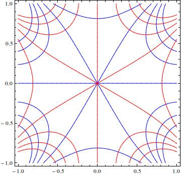
The function v also satisfies the Laplace equation, by a similar analysis. Also, the Cauchy–Riemann equations imply that the dot product ∇ u ⋅ ∇ v = 0 . This implies that the gradient of u must point along the v = const curves; so these are the streamlines of the flow. The u = const curves are the equipotential curves of the flow.

A holomorphic function can therefore be visualized by plotting the two families of level curves u = const and v = const . Near points where the gradient of u (or, equivalently, v) is not zero, these families form an orthogonal family of curves. At the points where ∇ u = 0 , the stationary points of the flow, the equipotential curves of u = const intersect. The streamlines also intersect at the same point, bisecting the angles formed by the equipotential curves.

Harmonic vector field

Another interpretation of the Cauchy–Riemann equations can be found in Pólya & Szegő (1978). Suppose that u and v satisfy the Cauchy–Riemann equations in an open subset of R², and consider the vector field

f ¯ = [ u − v ]

regarded as a (real) two-component vector. Then the second Cauchy–Riemann equation (1b) asserts that f ¯ is irrotational (its curl is 0):

∂ ( − v ) ∂ x − ∂ u ∂ y = 0.

The first Cauchy–Riemann equation (1a) asserts that the vector field is solenoidal (or divergence-free):

∂ u ∂ x + ∂ ( − v ) ∂ y = 0.

Owing respectively to Green's theorem and the divergence theorem, such a field is necessarily a conservative one, and it is free from sources or sinks, having net flux equal to zero through any open domain without holes. (These two observations combine as real and imaginary parts in Cauchy's integral theorem.) In fluid dynamics, such a vector field is a potential flow (Chanson 2007). In magnetostatics, such vector fields model static magnetic fields on a region of the plane containing no current. In electrostatics, they model static electric fields in a region of the plane containing no electric charge.

This interpretation can equivalently be restated in the language of differential forms. The pair u,v satisfy the Cauchy–Riemann equations if and only if the one-form v d x + u d y is both closed and coclosed (a harmonic differential form).

Preservation of complex structure

Another formulation of the Cauchy–Riemann equations involves the complex structure in the plane, given by

J = [ 0 1 − 1 0 ] .

This is a complex structure in the sense that the square of J is the negative of the 2×2 identity matrix: J 2 = − I . As above, if u(x,y),v(x,y) are two functions in the plane, put

f ( x , y ) = [ u ( x , y ) v ( x , y ) ] .

The Jacobian matrix of f is the matrix of partial derivatives

D f ( x , y ) = [ ∂ u ∂ x ∂ u ∂ y ∂ v ∂ x ∂ v ∂ y ]

Then the pair of functions u, v satisfies the Cauchy–Riemann equations if and only if the 2×2 matrix Df commutes with J (Kobayashi & Nomizu 1969, Proposition IX.2.2)

This interpretation is useful in symplectic geometry, where it is the starting point for the study of pseudoholomorphic curves.

Other representations

Other representations of the Cauchy–Riemann equations occasionally arise in other coordinate systems. If (1a) and (1b) hold for a differentiable pair of functions u and v, then so do

∂ u ∂ n = ∂ v ∂ s , ∂ v ∂ n = − ∂ u ∂ s

for any coordinate system (n(x, y), s(x, y)) such that the pair (∇n, ∇s) is orthonormal and positively oriented. As a consequence, in particular, in the system of coordinates given by the polar representation z = r e^iθ, the equations then take the form

∂ u ∂ r = 1 r ∂ v ∂ θ , ∂ v ∂ r = − 1 r ∂ u ∂ θ .

Combining these into one equation for f gives

∂ f ∂ r = 1 i r ∂ f ∂ θ .

The inhomogeneous Cauchy–Riemann equations consist of the two equations for a pair of unknown functions u(x,y) and v(x,y) of two real variables

∂ u ∂ x − ∂ v ∂ y = α ( x , y ) ∂ u ∂ y + ∂ v ∂ x = β ( x , y )

for some given functions α(x,y) and β(x,y) defined in an open subset of R². These equations are usually combined into a single equation

∂ f ∂ z ¯ = φ ( z , z ¯ )

where f = u + iv and φ = (α + iβ)/2.

If φ is C^k, then the inhomogeneous equation is explicitly solvable in any bounded domain D, provided φ is continuous on the closure of D. Indeed, by the Cauchy integral formula,

f ( ζ , ζ ¯ ) = 1 2 π i ∬ D φ ( z , z ¯ ) d z ∧ d z ¯ z − ζ

for all ζ ∈ D.

Goursat's theorem and its generalizations

Suppose that f = u + iv is a complex-valued function which is differentiable as a function f : R² → R². Then Goursat's theorem asserts that f is analytic in an open complex domain Ω if and only if it satisfies the Cauchy–Riemann equation in the domain (Rudin 1966, Theorem 11.2). In particular, continuous differentiability of f need not be assumed (Dieudonné 1969, §9.10, Ex. 1).

The hypotheses of Goursat's theorem can be weakened significantly. If f = u + iv is continuous in an open set Ω and the partial derivatives of f with respect to x and y exist in Ω, and satisfy the Cauchy–Riemann equations throughout Ω, then f is holomorphic (and thus analytic). This result is the Looman–Menchoff theorem.

The hypothesis that f obey the Cauchy–Riemann equations throughout the domain Ω is essential. It is possible to construct a continuous function satisfying the Cauchy–Riemann equations at a point, but which is not analytic at the point (e.g., f(z) = z⁵ / |z|⁴). Similarly, some additional assumption is needed besides the Cauchy–Riemann equations (such as continuity), as the following example illustrates (Looman 1923, p. 107)

f ( z ) = { exp ⁡ ( − z − 4 ) if  z ≠ 0 0 if  z = 0

which satisfies the Cauchy–Riemann equations everywhere, but fails to be continuous at z = 0.

Nevertheless, if a function satisfies the Cauchy–Riemann equations in an open set in a weak sense, then the function is analytic. More precisely (Gray & Morris 1978, Theorem 9):

If f(z) is locally integrable in an open domain Ω ⊂ C, and satisfies the Cauchy–Riemann equations weakly, then f agrees almost everywhere with an analytic function in Ω.

This is in fact a special case of a more general result on the regularity of solutions of hypoelliptic partial differential equations.

Several variables

There are Cauchy–Riemann equations, appropriately generalized, in the theory of several complex variables. They form a significant overdetermined system of PDEs. As often formulated, the d-bar operator

∂ ¯

annihilates holomorphic functions. This generalizes most directly the formulation

∂ f ∂ z ¯ = 0 ,

where

∂ f ∂ z ¯ = 1 2 ( ∂ f ∂ x + i ∂ f ∂ y ) .

Bäcklund transform

Viewed as conjugate harmonic functions, the Cauchy–Riemann equations are a simple example of a Bäcklund transform. More complicated, generally non-linear Bäcklund transforms, such as in the sine-Gordon equation, are of great interest in the theory of solitons and integrable systems.

Definition in Clifford algebra

In Clifford algebra the complex number z = x + i y is represented as z ≡ x + I y where I ≡ σ 1 σ 2 . The fundamental derivative operator in Clifford algebra of Complex numbers is defined as ∇ ≡ σ 1 ∂ x + σ 2 ∂ y . The function f = u + I v is considered analytic if and only if ∇ f = 0 , which can be calculated in following way:

0 = ∇ f = ( σ 1 ∂ x + σ 2 ∂ y ) ( u + σ 1 σ 2 v ) = σ 1 ∂ x u + σ 1 σ 1 σ 2 ⏟ = σ 2 ∂ x v + σ 2 ∂ y u + σ 2 σ 1 σ 2 ⏟ = − σ 1 ∂ y v = 0

Grouping by σ 1 and σ 2 :

∇ f = σ 1 ( ∂ x u − ∂ y v ) + σ 2 ( ∂ x v + ∂ y u ) = 0 ⇔ { ∂ x u − ∂ y v = 0 ∂ x v + ∂ y u = 0

Henceforth in traditional notation:

{ ∂ u ∂ x = ∂ v ∂ y ∂ u ∂ y = − ∂ v ∂ x

Conformal mappings in higher dimensions

Let Ω be an open set in the Euclidean space Rⁿ. The equation for an orientation-preserving mapping f : Ω → R n to be a conformal mapping (that is, angle-preserving) is that

D f T D f = ( det ( D f ) ) 2 / n I

where Df is the Jacobian matrix, with transpose D f T , and I denotes the identity matrix (Iwaniec & Martin 2001, p. 32). For n = 2, this system is equivalent to the standard Cauchy–Riemann equations of complex variables, and the solutions are holomorphic functions. In dimension n > 2, this is still sometimes called the Cauchy–Riemann system, and Liouville's theorem implies, under suitable smoothness assumptions, that any such mapping is a Möbius transformation.