Closed and exact differential forms

Examples

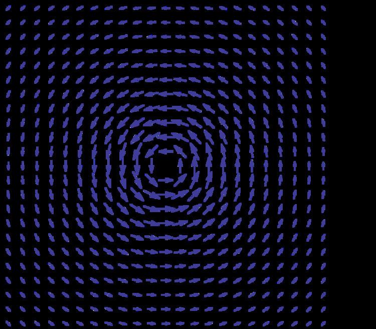
The simplest example of a form which is closed but not exact is the 1-form "dθ" (quotes because it is not the derivative of a globally defined function), defined on the punctured plane R 2 ∖ { 0 } , which is locally given as the derivative of the argument—note that argument is locally but not globally defined, since a loop around the origin increases (or decreases, depending on direction) the argument by 2π, which corresponds to the integral:

and for general paths is known as the winding number. The differential of the argument is however globally defined (except at the origin), since differentiation only requires local data and different values of the argument differ by a constant, so the derivatives of different local definitions are equal; this line of thought is generalized in the notion of covering spaces.

Explicitly, the form is given as:

which is not defined at the origin. This can be computed from a formula for the argument, most simply via arctan(y/x) (y/x is the slope of the line passing through (x,y), and arctan converts slope to angle), recognizing 1/(x²+y²) as corresponding to the derivative of arctan, which is 1/(x²+1) (these agree on the line y=1). While the differential is correctly computed by symbolically differentiating this expression, this formula is only strictly correct on the halfplane x>0, and properly one must use a correct formula for the argument.

This form generates the de Rham cohomology group H d R 1 ( R 2 ∖ { 0 } ) ≅ R , meaning that any closed form ω is the sum of an exact form d f and a multiple of d θ : ω = d f + k ⋅ d θ , where k = 1 2 π ∮ S 1 ω accounts for a non-trivial contour integral around the origin, which is the only obstruction to a closed form on the punctured plane (locally the derivative of a potential function) being the derivative of a globally defined function.

Examples in low dimensions

Differential forms in R² and R³ were well known in the mathematical physics of the nineteenth century. In the plane, 0-forms are just functions, and 2-forms are functions times the basic area element dx∧dy, so that it is the 1-forms

that are of real interest. The formula for the exterior derivative d here is

where the subscripts denote partial derivatives. Therefore the condition for α to be closed is

In this case if h(x,y) is a function then

The implication from 'exact' to 'closed' is then a consequence of the symmetry of second derivatives, with respect to x and y.

The gradient theorem asserts that a 1-form is exact if and only if the line integral of the form depends only on the endpoints of the curve, or equivalently, if the integral around any smooth closed curve is zero.

Vector field analogies

On a Riemannian manifold, or more generally a pseudo-Riemannian manifold, k-forms correspond to k-vector fields (by duality via the metric), so there is a notion of a vector field corresponding to a closed or exact form.

In 3 dimensions, an exact vector field (thought of as a 1-form) is called a conservative vector field, meaning that it is the derivative (gradient) of a 0-form (function), called the scalar potential. A closed vector field (thought of as a 1-form) is one whose derivative (curl) vanishes, and is called an irrotational vector field.

Thinking of a vector field as a 2-form instead, a closed vector field is one whose derivative (divergence) vanishes, and is called an incompressible flow (sometimes solenoidal vector field).

The concepts of conservative and incompressible vector fields generalize to n dimensions, because gradient and divergence generalize to n dimensions; curl is defined only in three dimensions, thus the concept of irrotational vector field does not generalize in this way.

Poincaré lemma

The Poincaré lemma states that if B is an open ball in Rⁿ, any smooth closed p-form ω defined on B is exact, for any integer p with 1 ≤ p ≤ n.

Translating if necessary, it can be assumed that the ball B has centre 0. Let α_s be the flow on Rⁿ defined by α_sx = e^−sx. For s ≤ 0 it carries B into itself and induces an action on functions and differential forms. The derivative of the flow is the vector field X defined on functions f by Xf = d(α_sf)/ds|_{s = 0}: it is the radial vector field r∂/∂r = ∑ x_i ∂/∂x_i. Often it is convenient to write the flow multiplicatively as a function of t = e^s, setting β_t = α_s, so that β_tx = t x. Only if 0 < t ≤ 1 will β_t carry B into itself. The derivative of the flow on forms defines the Lie derivative with respect to X given by L_X ω = d(α_sω) /ds|_s=0. In particular

so by the chain rule

Since α_s commutes with the exterior derivative d, so does the Lie derivative L_X. Moreover if ι_X denotes interior multiplication or contraction by the vector field X, then by Cartan's formula

Now define

Then h commutes with L_X, since L_X commutes with α_s and β_t. Furthermore h commutes with d. It also has the important property that

by the fundamental theorem of calculus since

Now set k = h ∘ ι_X. Then

Thus

(In the language of homological algebra, k is a "contracting homotopy".)

It now follows that if ω is closed, so that dω = 0, then d(kω) = (dk + kd)ω = ω, so that ω is exact and the Poincaré lemma is proved.

The same method applies to any open set in Rⁿ that is star-shaped about 0, i.e. any open set containing 0 and invariant under β_t for 0 < t < 1.

Example. In two dimensions the Poincaré lemma can be proved directly for closed 1-forms and 2-forms as follows.

If ω = p dx + q dy is a closed 1-form on (a,b) × (c,d), then p_y = q_x. If ω = df then p = f_x and q = f_y. Set

so that g_x = p. Then h = f − g must satisfy h_x = 0 and h_y = q − g_y. The right hand side here is independent of x since its partial derivative with respect to x is 0. So

and hence

Similarly if Ω = r dx ∧ dy then Ω = d(a dx + b dy) with b_x − a_y = r. Thus a solution is given by a = 0 and

Formulation as cohomology

When the difference of two closed forms is an exact form, they are said to be cohomologous to each other. That is, if ζ and η are closed forms, and one can find some β such that

then one says that ζ and η are cohomologous to each other. Exact forms are sometimes said to be cohomologous to zero. The set of all forms cohomologous to a given form (and thus to each other) is called a de Rham cohomology class; the general study of such classes is known as cohomology. It makes no real sense to ask whether a 0-form (smooth function) is exact, since d increases degree by 1; but the clues from topology suggest that only the zero function should be called "exact". The cohomology classes are identified with locally constant functions.

Using contracting homotopies similar to the one used in the proof of the Poincaré lemma, it can be shown that de Rham cohomology is homotopy-invariant. Non-contractible in general have non-trivial de Rham cohomology. For instance, on the circle S¹, parametrized by t in [0, 1], the closed 1-form dt is not exact.

Application in electrodynamics

In electrodynamics, the case of the magnetic field B → ( r ) produced by a stationary electrical current is important. There one deals with the vector potential A → ( r ) of this field. This case corresponds to k=2, and the defining region is the full R 3 . The current-density vector is j → . It corresponds to the current two-form

For the magnetic field B → one has analogous results: it corresponds to the induction two-form Φ B := B 1 d x 2 ∧ d x 3 + ⋯ , and can be derived from the vector potential A → , or the corresponding one-form A ,

Thereby the vector potential A → corresponds to the potential one-form

The closedness of the magnetic-induction two-form corresponds to the property of the magnetic field that it is source-free:   d i v B → ≡ 0 , i.e. there are no magnetic monopoles.

In a special gauge, d i v A → = ! 0 , this implies for i = 1, 2, 3

(Here μ 0 is a constant, the magnetic vacuum permeability.)

This equation is remarkable, because it corresponds completely to a well-known formula for the electrical field E → , namely for the electrostatic Coulomb potential ϕ ( x 1 , x 2 , x 3 ) of a charge density ρ ( x 1 , x 2 , x 3 ) . At this place one can already guess that

can be unified to quantities with six rsp. four nontrivial components, which is the basis of the relativistic invariance of the Maxwell equations.

If the condition of stationarity is left, on the l.h.s. of the above-mentioned equation one must add, in the equations for A i , to the three space coordinates, as a fourth variable also the time t, whereas on the r.h.s., in j i ′ , the so-called "retarded time",   t ′ := t − | r → − r → ′ | c , must be used, i.e. it is added to the argument of the current-density. Finally, as before, one integrates over the three primed space coordinates. (As usual c is the vacuum velocity of light.)