Divergence theorem

Intuition

If a fluid is flowing in some area, then the rate at which fluid flows out of a certain region within that area can be calculated by adding up the sources inside the region and subtracting the sinks. The fluid flow is represented by a vector field, and the vector field's divergence at a given point describes the strength of the source or sink there. So, integrating the field's divergence over the interior of the region should equal the integral of the vector field over the region's boundary. The divergence theorem says that this is true.

The divergence theorem is employed in any conservation law which states that the volume total of all sinks and sources, that is the volume integral of the divergence, is equal to the net flow across the volume's boundary.

Mathematical statement

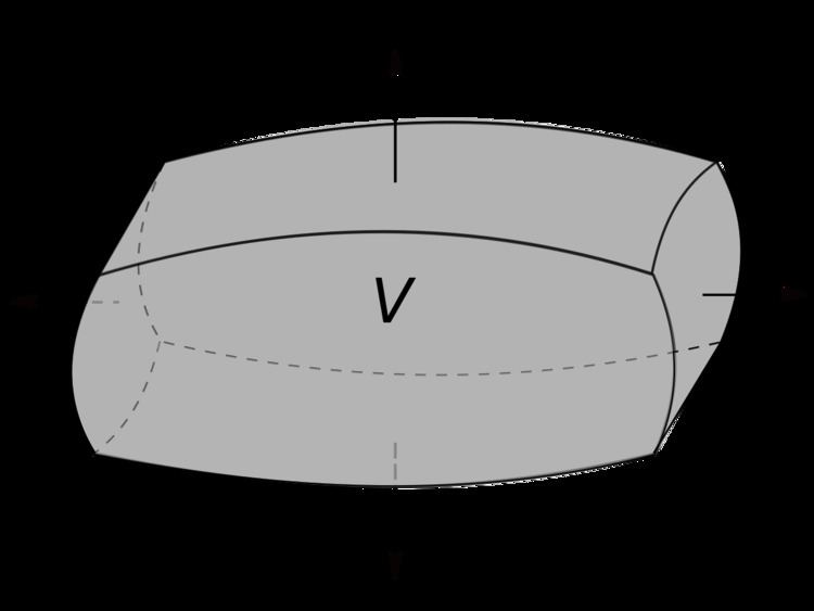
Suppose V is a subset of R n (in the case of n = 3, V represents a volume in 3D space) which is compact and has a piecewise smooth boundary S (also indicated with ∂V = S ). If F is a continuously differentiable vector field defined on a neighborhood of V, then we have:

∭ V ( ∇ ⋅ F ) d V = S ( F ⋅ n ) d S .

The left side is a volume integral over the volume V, the right side is the surface integral over the boundary of the volume V. The closed manifold ∂V is quite generally the boundary of V oriented by outward-pointing normals, and n is the outward pointing unit normal field of the boundary ∂V. (dS may be used as a shorthand for ndS.) The symbol within the two integrals stresses once more that ∂V is a closed surface. In terms of the intuitive description above, the left-hand side of the equation represents the total of the sources in the volume V, and the right-hand side represents the total flow across the boundary S.

Corollaries

By replacing F in the divergence theorem with specific forms, other useful identities can be derived (cf. vector identities).

With F → F g for a scalar function g and a vector field F,

A special case of this is F = ∇ f , in which case the theorem is the basis for Green's identities.

With F → F × G for two vector fields F and G,

With F → f c for a scalar function  f  and vector field c:

With F → c × F for vector field F and constant vector c:

Example

Suppose we wish to evaluate

S F ⋅ n d S ,

where S is the unit sphere defined by

S = { ( x , y , z ) ∈ R 3   :   x 2 + y 2 + z 2 = 1 } ,

and F is the vector field

F = 2 x i + y 2 j + z 2 k .

The direct computation of this integral is quite difficult, but we can simplify the derivation of the result using the divergence theorem, because the divergence theorem says that the integral is equal to:

∭ W ( ∇ ⋅ F ) d V = 2 ∭ W ( 1 + y + z ) d V = 2 ∭ W d V + 2 ∭ W y d V + 2 ∭ W z d V ,

where W is the unit ball:

W = { ( x , y , z ) ∈ R 3   :   x 2 + y 2 + z 2 ≤ 1 } .

Since the function y is positive in one hemisphere of W and negative in the other, in an equal and opposite way, its total integral over W is zero. The same is true for z:

∭ W y d V = ∭ W z d V = 0.

Therefore,

S F ⋅ n d S = 2 ∭ W d V = 8 π 3 ,

because the unit ball W has volume 4π/3.

Differential form and integral form of physical laws

As a result of the divergence theorem, a host of physical laws can be written in both a differential form (where one quantity is the divergence of another) and an integral form (where the flux of one quantity through a closed surface is equal to another quantity). Three examples are Gauss's law (in electrostatics), Gauss's law for magnetism, and Gauss's law for gravity.

Continuity equations

Continuity equations offer more examples of laws with both differential and integral forms, related to each other by the divergence theorem. In fluid dynamics, electromagnetism, quantum mechanics, relativity theory, and a number of other fields, there are continuity equations that describe the conservation of mass, momentum, energy, probability, or other quantities. Generically, these equations state that the divergence of the flow of the conserved quantity is equal to the distribution of sources or sinks of that quantity. The divergence theorem states that any such continuity equation can be written in a differential form (in terms of a divergence) and an integral form (in terms of a flux).

Inverse-square laws

Any inverse-square law can instead be written in a Gauss' law-type form (with a differential and integral form, as described above). Two examples are Gauss' law (in electrostatics), which follows from the inverse-square Coulomb's law, and Gauss' law for gravity, which follows from the inverse-square Newton's law of universal gravitation. The derivation of the Gauss' law-type equation from the inverse-square formulation (or vice versa) is exactly the same in both cases; see either of those articles for details.

History

The theorem was first discovered by Lagrange in 1762, then later independently rediscovered by Gauss in 1813, by Ostrogradsky, who also gave the first proof of the general theorem, in 1826, by Green in 1828, etc. Subsequently, variations on the divergence theorem are correctly called Ostrogradsky's theorem, but also commonly Gauss's theorem, or Green's theorem.

Examples

To verify the planar variant of the divergence theorem for a region R:

R = { ( x , y ) ∈ R 2   :   x 2 + y 2 ≤ 1 } ,

and the vector field:

F ( x , y ) = 2 y i + 5 x j .

The boundary of R is the unit circle, C, that can be represented parametrically by:

x = cos ⁡ ( s ) , y = sin ⁡ ( s )

such that 0 ≤ s ≤ 2π where s units is the length arc from the point s = 0 to the point P on C. Then a vector equation of C is

C ( s ) = cos ⁡ ( s ) i + sin ⁡ ( s ) j .

At a point P on C:

P = ( cos ⁡ ( s ) , sin ⁡ ( s ) ) ⇒ F = 2 sin ⁡ ( s ) i + 5 cos ⁡ ( s ) j .

Therefore,

∮ C F ⋅ n d s = ∫ 0 2 π ( 2 sin ⁡ ( s ) i + 5 cos ⁡ ( s ) j ) ⋅ ( cos ⁡ ( s ) i + sin ⁡ ( s ) j ) d s = ∫ 0 2 π ( 2 sin ⁡ ( s ) cos ⁡ ( s ) + 5 sin ⁡ ( s ) cos ⁡ ( s ) ) d s = 7 ∫ 0 2 π sin ⁡ ( s ) cos ⁡ ( s ) d s = 0.

Because M = 2y, ∂M/∂x = 0, and because N = 5x, ∂N/∂y = 0. Thus

∬ R ∇ ⋅ F d A = ∬ R ( ∂ M ∂ x + ∂ N ∂ y ) d A = 0.

Multiple dimensions

One can use the general Stokes' Theorem to equate the n-dimensional volume integral of the divergence of a vector field F over a region U to the (n − 1)-dimensional surface integral of F over the boundary of U:

∫ ⋯ ∫ U ⏟ n ∇ ⋅ F d V = ∮ ⋯ ∮ ∂ U ⏟ n − 1 F ⋅ n d S

This equation is also known as the Divergence theorem.

When n = 2, this is equivalent to Green's theorem.

When n = 1, it reduces to the Fundamental theorem of calculus.

Tensor fields

Writing the theorem in Einstein notation:

∭ V ∂ F i ∂ x i d V = S F i n i d S

suggestively, replacing the vector field F with a rank-n tensor field T, this can be generalized to:

∭ V ∂ T i 1 i 2 ⋯ i q ⋯ i n ∂ x i q d V = S T i 1 i 2 ⋯ i q ⋯ i n n i q d S .

where on each side, tensor contraction occurs for at least one index. This form of the theorem is still in 3d, each index takes values 1, 2, and 3. It can be generalized further still to higher (or lower) dimensions (for example to 4d spacetime in general relativity).