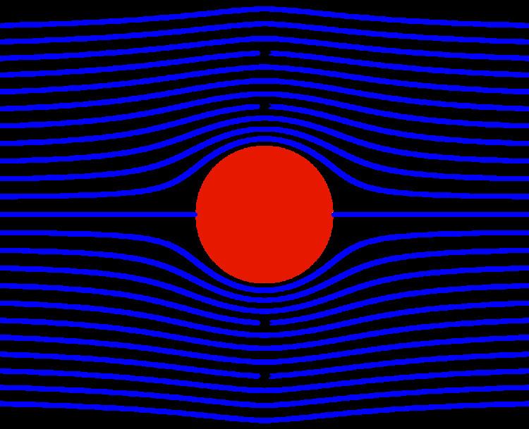
Stream function - Alchetron, The Free Social Encyclopedia

The stream function is defined for incompressible (divergence-free) flows in two dimensions – as well as in three dimensions with axisymmetry. The flow velocity components can then be expressed as the derivatives of the scalar stream function. The stream function can be used to plot streamlines, which represent the trajectories of particles in a steady flow. The two-dimensional Lagrange stream function was introduced by Joseph Louis Lagrange in 1781. The Stokes stream function is for axisymmetrical three-dimensional flow, and is named after George Gabriel Stokes.

Since streamlines are tangent to the flow velocity vector of the flow, the value of the stream function must be constant along a streamline. The usefulness of the stream function lies in the fact that the flow velocity components in the x- and y- directions at a given point are given by the partial derivatives of the stream function at that point. A stream function may be defined for any flow of dimensions greater than or equal to two, however the two-dimensional case is generally the easiest to visualize and derive.

For two-dimensional potential flow, streamlines are perpendicular to equipotential lines. Taken together with the velocity potential, the stream function may be used to derive a complex potential. In other words, the stream function accounts for the solenoidal part of a two-dimensional Helmholtz decomposition, while the velocity potential accounts for the irrotational part.

Definitions

Lamb and Batchelor define the stream function ψ ( x , y , t ) – in the point P with two-dimensional coordinates ( x , y ) and as a function of time t – for an incompressible flow by:

ψ = ∫ A P ( u d y − v d x ) .

So the stream function ψ is the volume flux through the curve A P , that is: the integral of the dot product of the flow velocity vector ( u , v ) and the normal ( + d y , − d x ) to the curve element ( d x , d y ) . The point A is a reference point defining where the stream function is zero: a shift of A results in adding a constant to the stream function ψ .

An infinitesimal shift δ P = ( δ x , δ y ) of the position P results in a stream function shift:

δ ψ = u δ y − v δ x ,

which is an exact differential provided

∂ u ∂ x + ∂ v ∂ y = 0.

This is the condition of zero divergence resulting from flow incompressibility. Since

δ ψ = ∂ ψ ∂ x δ x + ∂ ψ ∂ y δ y ,

the flow velocity components have to be

u = + ∂ ψ ∂ y and v = − ∂ ψ ∂ x

in relation to the stream function ψ .

Definition by use of a vector potential

The sign of the stream function depends on the definition used.

One way is to define the stream function ψ for a two-dimensional flow such that the flow velocity can be expressed through the vector potential ψ :

u = ∇ × ψ

Where ψ = ( 0 , 0 , ψ ) if the flow velocity vector u = ( u , v , 0 ) .

In Cartesian coordinate system this is equivalent to

u = ∂ ψ ∂ y , v = − ∂ ψ ∂ x

Where u and v are the flow velocity components in the cartesian x and y coordinate directions, respectively.

Alternative definition (opposite sign)

Another definition (used more widely in meteorology and oceanography than the above) is

u = z × ∇ ψ ′ ≡ ( − ψ y ′ , ψ x ′ , 0 ) ,

where z = ( 0 , 0 , 1 ) is a unit vector in the + z direction and the subscripts indicate partial derivatives.

Note that this definition has the opposite sign to that given above ( ψ ′ = − ψ ), so we have

u = − ∂ ψ ′ ∂ y , v = ∂ ψ ′ ∂ x

in Cartesian coordinates.

All formulations of the stream function constrain the velocity to satisfy the two-dimensional continuity equation exactly:

∂ u ∂ x + ∂ v ∂ y = 0

The last two definitions of stream function are related through the vector calculus identity

∇ × ( ψ z ) = ψ ∇ × z + ∇ ψ × z = ∇ ψ × z = z × ∇ ψ ′ .

Note that ψ = ψ z in this two-dimensional flow.

Derivation of the two-dimensional stream function

Consider two points A and B in two-dimensional plane flow. If the distance between these two points is very small: δn, and a stream of flow passes between these points with an average velocity, q perpendicular to the line AB, the volume flow rate per unit thickness, δΨ is given by:

δ ψ = q δ n

As δn → 0, rearranging this expression, we get:

q = ∂ ψ ∂ n

Now consider two-dimensional plane flow with reference to a coordinate system. Suppose an observer looks along an arbitrary axis in the direction of increase and sees flow crossing the axis from left to right. A sign convention is adopted such that the flow velocity is positive.

Flow in Cartesian coordinates

By observing the flow into an elemental square in an x-y Cartesian coordinate system, we have:

δ ψ = u δ y δ ψ = − v δ x

where u is the flow velocity parallel to and in the direction of the x-axis, and v is the flow velocity parallel to and in the direction of the y-axis. Thus, as δn → 0 and by rearranging, we have:

u = ∂ ψ ∂ y v = − ∂ ψ ∂ x

Continuity: the derivation

Consider two-dimensional plane flow within a Cartesian coordinate system. Continuity states that if we consider incompressible flow into an elemental square, the flow into that small element must equal the flow out of that element.

The total flow into the element is given by:

δ ψ i n = u δ y + v δ x .

The total flow out of the element is given by:

δ ψ o u t = ( u + ∂ u ∂ x δ x ) δ y + ( v + ∂ v ∂ y δ y ) δ x .

Thus we have:

δ ψ i n = δ ψ o u t u δ y + v δ x = ( u + ∂ u ∂ x δ x ) δ y + ( v + ∂ v ∂ y δ y ) δ x

and simplifying to:

∂ u ∂ x + ∂ v ∂ y = 0.

Substituting the expressions of the stream function into this equation, we have:

∂ 2 ψ ∂ x ∂ y − ∂ 2 ψ ∂ y ∂ x = 0.

Vorticity

The stream function can be found from vorticity using the following Poisson's equation:

∇ 2 ψ = − ω

or

∇ 2 ψ ′ = + ω

where the vorticity vector ω = ∇ × u – defined as the curl of the flow velocity vector u – for this two-dimensional flow has ω = ( 0 , 0 , ω ) , i.e. only the z -component ω can be non-zero.

Proof that a constant value for the stream function corresponds to a streamline

Consider two-dimensional plane flow within a Cartesian coordinate system. Consider two infinitesimally close points P = ( x , y ) and Q = ( x + d x , y + d y ) . From calculus we have that

ψ ( x + d x , y + d y ) − ψ ( x , y ) = ∂ ψ ∂ x d x + ∂ ψ ∂ y d y = ∇ ψ ⋅ d r

Say ψ takes the same value, say C , at the two points P and Q , then d r is tangent to the curve ψ = C at P and

0 = ψ ( x + d x , y + d y ) − ψ ( x , y ) = ∇ ψ ⋅ d r

implying that the vector ∇ ψ is normal to the curve ψ = C . If we can show that everywhere u ⋅ ∇ ψ = 0 , using the formula for u in terms of ψ , then we will have proved the result. This easily follows,

u ⋅ ∇ ψ = ∂ ψ ∂ y ∂ ψ ∂ x + ( − ∂ ψ ∂ x ) ∂ ψ ∂ y = 0.

Properties of Stream Function

Stream function ψ is constant on any streamline.
For the continuous flow, the flow around any path is equal to zero.
For two incompressible flow patterns, the algebraic sum of the stream functions is equal to another stream function obtained if the two flow patterns are super-imposed.
The rate of change of stream function with distance is directly proportional to the velocity component perpendicular to the direction of change.

References

Stream function Wikipedia

(Text) CC BY-SA