
 | ||
Parameters α ∈ (0, 2] — stability parameterβ ∈ [−1, 1] — skewness parameter (note that skewness is undefined)c ∈ (0, ∞) — scale parameterμ ∈ (−∞, ∞) — location parameter Support x ∈ R, or x ∈ [μ, +∞) if α < 1 and β = 1, or x ∈ (-∞, μ] if α < 1 and β = −1 PDF not analytically expressible, except for some parameter values CDF not analytically expressible, except for certain parameter values Mean μ when α > 1, otherwise undefined Median μ when β = 0, otherwise not analytically expressible | ||
In probability theory, a distribution or a random variable is said to be stable if a linear combination of two independent copies of a random sample has the same distribution, up to location and scale parameters. The stable distribution family is also sometimes referred to as the Lévy alpha-stable distribution, after Paul Lévy, the first mathematician to have studied it.
Contents
- Definition
- Parametrizations
- The distribution
- Properties
- A generalized central limit theorem
- Special cases
- Series representation
- Simulation of stable variables
- Applications
- Other analytic cases
- References
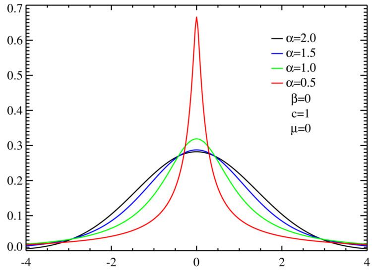
Of the four parameters defining the family, most attention has been focused on the stability parameter, α (see panel). Stable distributions have 0 < α ≤ 2, with the upper bound corresponding to the normal distribution, and α = 1 to the Cauchy distribution. The distributions have undefined variance for α < 2, and undefined mean for α ≤ 1. The importance of stable probability distributions is that they are "attractors" for properly normed sums of independent and identically-distributed (iid) random variables. The normal distribution defines a family of stable distributions. By the classical central limit theorem the properly normed sum of a set of random variables, each with finite variance, will tend towards a normal distribution as the number of variables increases. Without the finite variance assumption, the limit may be a stable distribution that is not normal. Mandelbrot referred to such distributions as "stable Paretian distributions", after Vilfredo Pareto. In particular, he referred to those maximally skewed in the positive direction with 1<α<2 as "Pareto-Lévy distributions", which he regarded as better descriptions of stock and commodity prices than normal distributions.
Definition
A non-degenerate distribution is a stable distribution if it satisfies the following property:
Let X1 and X2 be independent copies of a random variable X. Then X is said to be stable if for any constants a > 0 and b > 0 the random variable aX1 + bX2 has the same distribution as cX + d for some constants c > 0 and d. The distribution is said to be strictly stable if this holds with d = 0.Since the normal distribution, the Cauchy distribution, and the Lévy distribution all have the above property, it follows that they are special cases of stable distributions.
Such distributions form a four-parameter family of continuous probability distributions parametrized by location and scale parameters μ and c, respectively, and two shape parameters β and α, roughly corresponding to measures of asymmetry and concentration, respectively (see the figures).
Although the probability density function for a general stable distribution cannot be written analytically, the general characteristic function can be. Any probability distribution is given by the Fourier transform of its characteristic function φ(t) by:
A random variable X is called stable if its characteristic function can be written as
where sgn(t) is just the sign of t and
μ ∈ R is a shift parameter, β ∈ [−1, 1], called the skewness parameter, is a measure of asymmetry. Notice that in this context the usual skewness is not well defined, as for α < 2 the distribution does not admit 2nd or higher moments, and the usual skewness definition is the 3rd central moment.
The reason this gives a stable distribution is that the characteristic function for the sum of two random variables equals the product of the two corresponding characteristic functions. Adding two random variables from a stable distribution gives something with the same values of α and β, but possibly different values of μ and c.
Not every function is the characteristic function of a legitimate probability distribution (that is, one whose cumulative distribution function is real and goes from 0 to 1 without decreasing), but the characteristic functions given above will be legitimate so long as the parameters are in their ranges. The value of the characteristic function at some value t is the complex conjugate of its value at −t as it should be so that the probability distribution function will be real.
In the simplest case β = 0, the characteristic function is just a stretched exponential function; the distribution is symmetric about μ and is referred to as a (Lévy) symmetric alpha-stable distribution, often abbreviated SαS.
When α < 1 and β = 1, the distribution is supported by [μ, ∞).
The parameter c > 0 is a scale factor which is a measure of the width of the distribution while α is the exponent or index of the distribution and specifies the asymptotic behavior of the distribution.
Parametrizations
The above definition is only one of the parametrizations in use for stable distributions; it is the most common but is not continuous in the parameters at α = 1.
A continuous parametrization is
where:
The ranges of α and β are the same as before, γ (like c) should be positive, and δ (like μ) should be real.
In either parametrization one can make a linear transformation of the random variable to get a random variable whose density is
For the second parametrization, we simply use
no matter what α is. In the first parametrization, if the mean exists (that is, α > 1) then it is equal to μ, whereas in the second parametrization when the mean exists it is equal to
The distribution
A stable distribution is therefore specified by the above four parameters. It can be shown that any non-degenerate stable distribution has a smooth (infinitely differentiable) density function. If
then Y has the density
The asymptotic behavior is described, for α< 2, by:
where Γ is the Gamma function (except that when α < 1 and β = ±1, the tail vanishes to the left or right, resp., of μ). This "heavy tail" behavior causes the variance of stable distributions to be infinite for all α < 2. This property is illustrated in the log-log plots below.
When α = 2, the distribution is Gaussian (see below), with tails asymptotic to exp(−x2/4c2)/(2c√π).
Properties
Stable distributions are closed under convolution for a fixed value of α. Since convolution is equivalent to multiplication of the Fourier-transformed function, it follows that the product of two stable characteristic functions with the same α will yield another such characteristic function. The product of two stable characteristic functions is given by:
Since Φ is not a function of the μ, c or β variables it follows that these parameters for the convolved function are given by:
In each case, it can be shown that the resulting parameters lie within the required intervals for a stable distribution.
A generalized central limit theorem
Another important property of stable distributions is the role that they play in a generalized central limit theorem. The central limit theorem states that the sum of a number of independent and identically distributed (i.i.d.) random variables with finite variances will tend to a normal distribution as the number of variables grows.
A generalization due to Gnedenko and Kolmogorov states that the sum of a number of random variables with symmetric distributions having power-law tails (Paretian tails), decreasing as |x|−α−1 where 0 < α < 2 (and therefore having infinite variance), will tend to a stable distribution
There are other possibilities as well. For example, if the characteristic function of the random variable is asymptotic to
Assuming for the moment that t tends toward zero, we take the limit of the above as n → ∞:
This shows that
This implies that the sum divided by
This can be applied to a random variable whose tails decrease as
We can write this as
where:
We want to find the leading terms of the asymptotic expansion of the characteristic function. The characteristic function of the probability distribution
and we have
The term in brackets is asymptotic to
and we may break the integral into several parts. The first part is the integral of the leading term from w = 1 out to w = 1/|t|, the second term is the integral of the remainder, going from zero to 1/|t|, the third term subtracts out the integral of the same but from 0 to 1, and the last term is the integral from 1/|t| to infinity:
Therefore
and according to what was said above (and the fact that the variance of f(x;2,0,1,0) is 2), the sum of n instances of this random variable, divided by
Special cases
There is no general analytic solution for the form of p(x). There are, however three special cases which can be expressed in terms of elementary functions as can be seen by inspection of the characteristic function:
Note that the above three distributions are also connected, in the following way: A standard Cauchy random variable can be viewed as a mixture of Gaussian random variables (all with mean zero), with the variance being drawn from a standard Lévy distribution. And in fact this is a special case of a more general theorem which allows any symmetric alpha-stable distribution to be viewed in this way (with the alpha parameter of the mixture distribution equal to twice the alpha parameter of the mixing distribution—and the beta parameter of the mixing distribution always equal to one).
A general closed form expression for stable PDF's with rational values of α is available in terms of Meijer G-functions. Fox H-Functions can also be used to express the stable probability density functions. For simple rational numbers, the closed form expression is often in terms of less complicated special functions. Several closed form expressions having rather simple expressions in terms of special functions are available. In the table below, PDF's expressible by elementary functions are indicated by an E and those that are expressible by special functions are indicated by an s.
Some of the special cases are known by particular names:
Also, in the limit as c approaches zero or as α approaches zero the distribution will approach a Dirac delta function δ(x − μ).
Series representation
The stable distribution can be restated as the real part of a simpler integral:
Expressing the second exponential as a Taylor series, we have:
where
which will be valid for x ≠ μ and will converge for appropriate values of the parameters. (Note that the n = 0 term which yields a delta function in x−μ has therefore been dropped.) Expressing the first exponential as a series will yield another series in positive powers of x−μ which is generally less useful.
Simulation of stable variables
Simulating sequences of stable random variables is not straightforward, since there are no analytic expressions for the inverse
This algorithm yields a random variable
Given the formulas for simulation of a standard stable random variable, we can easily simulate a stable random variable for all admissible values of the parameters
is
Applications
Stable distributions owe their importance in both theory and practice to the generalization of the central limit theorem to random variables without second (and possibly first) order moments and the accompanying self-similarity of the stable family. It was the seeming departure from normality along with the demand for a self-similar model for financial data (i.e. the shape of the distribution for yearly asset price changes should resemble that of the constituent daily or monthly price changes) that led Benoît Mandelbrot to propose that cotton prices follow an alpha-stable distribution with α equal to 1.7. Lévy distributions are frequently found in analysis of critical behavior and financial data.
They are also found in spectroscopy as a general expression for a quasistatically pressure broadened spectral line.
The Lévy distribution of solar flare waiting time events (time between flare events) was demonstrated for CGRO BATSE hard x-ray solar flares in December 2001. Analysis of the Lévy statistical signature revealed that two different memory signatures were evident; one related to the solar cycle and the second whose origin appears to be associated with a localized or combination of localized solar active region effects.
Other analytic cases
A number of cases of analytically expressible stable distributions are known. Let the stable distribution be expressed by