Suvarna Garge (Editor)

Holtsmark distribution

Updated on
Edit
Like
Comment
Share on FacebookTweet on TwitterShare on LinkedInShare on Reddit
Support
  
x ∈ R

Median
  
μ

Mean
  
μ

Mode
  
μ

Holtsmark distribution

Parameters
  
c ∈ (0, ∞) — scale parameter μ ∈ (−∞, ∞) — location parameter

PDF
  
expressible in terms of hypergeometric functions; see text

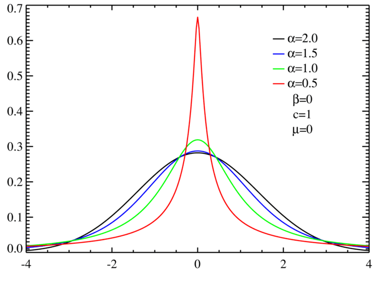
The (one-dimensional) Holtsmark distribution is a continuous probability distribution. The Holtsmark distribution is a special case of a stable distribution with the index of stability or shape parameter α equal to 3/2 and skewness parameter β of zero. Since β equals zero, the distribution is symmetric, and thus an example of a symmetric alpha-stable distribution. The Holtsmark distribution is one of the few examples of a stable distribution for which a closed form expression of the probability density function is known. However, its probability density function is not expressible in terms of elementary functions; rather, the probability density function is expressed in terms of hypergeometric functions.

Contents

The Holtsmark distribution has applications in plasma physics and astrophysics. In 1919, Norwegian physicist J. Holtsmark proposed the distribution as a model for the fluctuating fields in plasma due to chaotic motion of charged particles. It is also applicable to other types of Coulomb forces, in particular to modeling of gravitating bodies, and thus is important in astrophysics.

Characteristic function

The characteristic function of a symmetric stable distribution is:

φ ( t ; μ , c ) = exp [   i t μ | c t | α   ] ,

where α is the shape parameter, or index of stability, μ is the location parameter, and c is the scale parameter.

Since the Holtsmark distribution has α = 3 / 2 , its characteristic function is:

φ ( t ; μ , c ) = exp [   i t μ | c t | 3 / 2   ] .

Since the Holtsmark distribution is a stable distribution with α > 1, μ represents the mean of the distribution. Since β = 0, μ also represents the median and mode of the distribution. And since α < 2, the variance of the Holtsmark distribution is infinite. All higher moments of the distribution are also infinite. Like other stable distributions (other than the normal distribution), since the variance is infinite the dispersion in the distribution is reflected by the scale parameter, c. An alternate approach to describing the dispersion of the distribution is through fractional moments.

Probability density function

In general, the probability density function, f(x), of a continuous probability distribution can be derived from its characteristic function by:

f ( x ) = 1 2 π φ ( t ) e i x t d t .

Most stable distributions do not have a known closed form expression for their probability density functions. Only the normal, Cauchy and Lévy distributions have known closed form expressions in terms of elementary functions. The Holtsmark distribution is one of two symmetric stable distributions to have a known closed form expression in terms of hypergeometric functions. When μ is equal to 0 and the scale parameter is equal to 1, the Holtsmark distribution has the probability density function:

f ( x ; 0 , 1 ) = 1 π Γ ( 5 / 3 ) 2 F 3 ( 5 / 12 , 11 / 12 ; 1 / 3 , 1 / 2 , 5 / 6 ; 4 x 6 / 729 ) x 2 3 π 3 F 4 ( 3 / 4 , 1 , 5 / 4 ; 2 / 3 , 5 / 6 , 7 / 6 , 4 / 3 ; 4 x 6 / 729 ) + 7 x 4 81 π Γ ( 4 / 3 ) 2 F 3 ( 13 / 12 , 19 / 12 ; 7 / 6 , 3 / 2 , 5 / 3 ; 4 x 6 / 729 ) ,

where Γ ( x ) is the gamma function and m F n ( ) is a hypergeometric function.

References

Holtsmark distribution Wikipedia