Box–Muller transform - Alchetron, The Free Social Encyclopedia

The Box–Muller transform, by George Edward Pelham Box and Mervin Edgar Muller 1958, is a pseudo-random number sampling method for generating pairs of independent, standard, normally distributed (zero expectation, unit variance) random numbers, given a source of uniformly distributed random numbers.

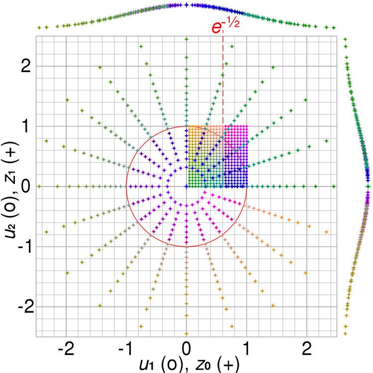
It is commonly expressed in two forms. The basic form as given by Box and Muller takes two samples from the uniform distribution on the interval [0, 1] and maps them to two standard, normally distributed samples. The polar form takes two samples from a different interval, [−1, +1], and maps them to two normally distributed samples without the use of sine or cosine functions.

The Box–Muller transform was developed as a more computationally efficient alternative to the inverse transform sampling method. The Ziggurat algorithm gives an even more efficient method. Furthermore, the Box–Muller transform can be employed for drawing from truncated bivariate Gaussian densities.

Basic form

Suppose U₁ and U₂ are independent random variables that are uniformly distributed in the interval (0, 1). Let

Z 0 = R cos ⁡ ( Θ ) = − 2 ln ⁡ U 1 cos ⁡ ( 2 π U 2 )

and

Z 1 = R sin ⁡ ( Θ ) = − 2 ln ⁡ U 1 sin ⁡ ( 2 π U 2 ) .

Then Z₀ and Z₁ are independent random variables with a standard normal distribution.

The derivation is based on a property of a two-dimensional Cartesian system, where X and Y coordinates are described by two independent and normally distributed random variables, the random variables for R² and Θ (shown above) in the corresponding polar coordinates are also independent and can be expressed as

R 2 = − 2 ⋅ ln ⁡ U 1

and

Θ = 2 π U 2 .

Because R² is the square of the norm of the standard bivariate normal variable (X, Y), it has the chi-squared distribution with two degrees of freedom. In the special case of two degrees of freedom, the chi-squared distribution coincides with the exponential distribution, and the equation for R² above is a simple way of generating the required exponential variate.

Polar form

The polar form was first proposed by J. Bell and then modified by R. Knop. While several different versions of the polar method have been described, the version of R. Knop will be described here because it is the most widely used, in part due to its inclusion in Numerical Recipes.

Given u and v, independent and uniformly distributed in the closed interval [−1, +1], set s = R² = u² + v². (Clearly R = s ). If s = 0 or s ≥ 1, discard u and v, and try another pair (u, v). Because u and v are uniformly distributed and because only points within the unit circle have been admitted, the values of s will be uniformly distributed in the open interval (0, 1), too. The latter can be seen by calculating the cumulative distribution function for s in the interval (0, 1). This is the area of a circle with radius s , divided by π . From this we find the probability density function to have the constant value 1 on the interval (0, 1). Equally so, the angle θ divided by 2 π is uniformly distributed in the interval [0, 1) and independent of s.

We now identify the value of s with that of U₁ and θ / ( 2 π ) with that of U₂ in the basic form. As shown in the figure, the values of cos ⁡ θ = cos ⁡ 2 π U 2 and sin ⁡ θ = sin ⁡ 2 π U 2 in the basic form can be replaced with the ratios cos ⁡ θ = u / R = u / s and sin ⁡ θ = v / R = v / s , respectively. The advantage is that calculating the trigonometric functions directly can be avoided. This is helpful when trigonometric functions are more expensive to compute than the single division that replaces each one.

Just as the basic form produces two standard normal deviates, so does this alternate calculation.

z 0 = − 2 ln ⁡ U 1 cos ⁡ ( 2 π U 2 ) = − 2 ln ⁡ s ( u s ) = u ⋅ − 2 ln ⁡ s s

and

z 1 = − 2 ln ⁡ U 1 sin ⁡ ( 2 π U 2 ) = − 2 ln ⁡ s ( v s ) = v ⋅ − 2 ln ⁡ s s .

Contrasting the two forms

The polar method differs from the basic method in that it is a type of rejection sampling. It discards some generated random numbers, but it is typically faster than the basic method because it is simpler to compute (provided that the random number generator is relatively fast) and is more numerically robust. It avoids the use of trigonometric functions, which are comparatively expensive in many computing environments. It discards 1 − π/4 ≈ 21.46% of the total input uniformly distributed random number pairs generated, i.e. discards 4/π − 1 ≈ 27.32% uniformly distributed random number pairs per Gaussian random number pair generated, requiring 4/π ≈ 1.2732 input random numbers per output random number.

The basic form requires two multiplications, 1/2 logarithm, 1/2 square root, and one trigonometric function for each normal variate. On some processors, the cosine and sine of the same argument can be calculated in parallel using a single instruction. Notably for Intel-based machines, one can use the fsincos assembler instruction or the expi instruction (usually available from C as an intrinsic function), to calculate complex

e x p ( i z ) = e i z = cos ⁡ ( z ) + i sin ⁡ ( z ) ,

and just separate the real and imaginary parts.

The polar form requires 3/2 multiplications, 1/2 logarithm, 1/2 square root, and 1/2 division for each normal variate. The effect is to replace one multiplication and one trigonometric function with a single division.

Tails truncation

When a computer is used to produce a uniform random variable it will inevitably have some inaccuracies because there is a lower bound on how close numbers can be to 0. If the generator uses 32 bits per output value, the smallest non-zero number that can be generated is 2 − 32 . When U 1 and U 2 are equal to this the Box–Muller transform produces a normal random variable equal to − 2 ln ⁡ ( 2 − 32 ) cos ⁡ ( 2 π 2 − 32 ) ≈ 6.66 This means that the algorithm will not produce random variables more than 6.66 standard deviations from the mean. This corresponds to a proportion of 2.74 × 10 − 11 lost due to the truncation.

Implementation

The standard Box–Muller transform generates values from the standard normal distribution (i.e. standard normal deviates) with mean 0 and standard deviation 1. The implementation below in standard C++ generates values from any normal distribution with mean μ and variance σ 2 . If Z is a standard normal deviate, then X = Z σ + μ will have a normal distribution with mean μ and standard deviation σ . Note that because the random number generator rand has not been seeded, the same series of values will always be returned from the generateGaussianNoise function.

References

Box–Muller transform Wikipedia

(Text) CC BY-SA