Supriya Ghosh (Editor)

Lévy distribution

Updated on
Edit
Like
Comment
Share on FacebookTweet on TwitterShare on LinkedInShare on Reddit
Lévy distribution

Parameters
  
μ {\displaystyle \mu } location; c > 0 {\displaystyle c>0\,} scale

Support
  
x ∈ [ μ , ∞ ) {\displaystyle x\in [\mu ,\infty )}

PDF
  
c 2 π     e − c 2 ( x − μ ) ( x − μ ) 3 / 2 {\displaystyle {\sqrt {\frac {c}{2\pi }}}~~{\frac {e^{-{\frac {c}{2(x-\mu )}}}}{(x-\mu )^{3/2}}}}

CDF
  
erfc ( c 2 ( x − μ ) ) {\displaystyle {\textrm {erfc}}\left({\sqrt {\frac {c}{2(x-\mu )}}}\right)}

Mean
  
∞ {\displaystyle \infty }

Median
  
c / 2 ( erfc − 1 ( 1 / 2 ) ) 2 {\displaystyle c/2({\textrm {erfc}}^{-1}(1/2))^{2}\,} , for μ = 0 {\displaystyle \mu =0}

In probability theory and statistics, the Lévy distribution, named after Paul Lévy, is a continuous probability distribution for a non-negative random variable. In spectroscopy, this distribution, with frequency as the dependent variable, is known as a van der Waals profile. It is a special case of the inverse-gamma distribution.

Contents

It is one of the few distributions that are stable and that have probability density functions that can be expressed analytically, the others being the normal distribution and the Cauchy distribution.

Definition

The probability density function of the Lévy distribution over the domain x μ is

f ( x ; μ , c ) = c 2 π     e c 2 ( x μ ) ( x μ ) 3 / 2

where μ is the location parameter and c is the scale parameter. The cumulative distribution function is

F ( x ; μ , c ) = erfc ( c 2 ( x μ ) )

where erfc ( z ) is the complementary error function. The shift parameter μ has the effect of shifting the curve to the right by an amount μ , and changing the support to the interval [ μ , ). Like all stable distributions, the Levy distribution has a standard form f(x;0,1) which has the following property:

f ( x ; μ , c ) d x = f ( y ; 0 , 1 ) d y

where y is defined as

y = x μ c

The characteristic function of the Lévy distribution is given by

φ ( t ; μ , c ) = e i μ t 2 i c t .

Note that the characteristic function can also be written in the same form used for the stable distribution with α = 1 / 2 and β = 1 :

φ ( t ; μ , c ) = e i μ t | c t | 1 / 2   ( 1 i   sign ( t ) ) .

Assuming μ = 0 , the nth moment of the unshifted Lévy distribution is formally defined by:

m n   = d e f   c 2 π 0 e c / 2 x x n x 3 / 2 d x

which diverges for all n > 0 so that the moments of the Lévy distribution do not exist. The moment generating function is then formally defined by:

M ( t ; c )   = d e f   c 2 π 0 e c / 2 x + t x x 3 / 2 d x

which diverges for t > 0 and is therefore not defined in an interval around zero, so that the moment generating function is not defined per se. Like all stable distributions except the normal distribution, the wing of the probability density function exhibits heavy tail behavior falling off according to a power law:

f ( x ; μ , c ) c 2 π 1 x 3 / 2   as   x .

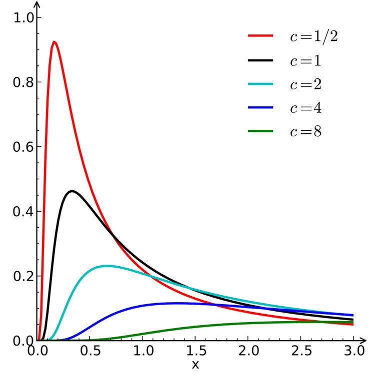
This is illustrated in the diagram below, in which the probability density functions for various values of c and μ = 0 are plotted on a log-log scale.

Differential equation

{ f ( x ) ( c 3 μ + 3 x ) + 2 ( x μ ) 2 f ( x ) = 0 , f ( 0 ) = e c 2 μ ( c μ ) 3 / 2 2 π c }

Properties

The standard Lévy distribution satisfies the condition

( X 1 + X 2 + + X n ) n 1 / α X ,

where X 1 , X 2 , , X n , X are standard Lévy-variables with α = 1 / 2 .

  • If X Levy ( μ , c ) then k X + b Levy ( k μ + b , k c )
  • If X Levy ( 0 , c ) then X Inv-Gamma ( 1 2 , c 2 ) (inverse gamma distribution)
  • Lévy distribution is a special case of type 5 Pearson distribution
  • If Y Normal ( μ , σ 2 ) (Normal distribution) then ( Y μ ) 2 Levy ( 0 , 1 / σ 2 )
  • If X Normal ( μ , 1 σ ) then ( X μ ) 2 Levy ( 0 , σ )
  • If X Levy ( μ , c ) then X Stable ( 1 / 2 , 1 , c , μ ) (Stable distribution)
  • If X Levy ( 0 , c ) then X Scale-inv- χ 2 ( 1 , c ) (Scaled-inverse-chi-squared distribution)
  • If X Levy ( μ , c ) then ( X μ ) 1 2 FoldedNormal ( 0 , 1 / c ) (Folded normal distribution)
  • Random sample generation

    Random samples from the Lévy distribution can be generated using inverse transform sampling. Given a random variate U drawn from the uniform distribution on the unit interval (0, 1], the variate X given by

    X = F 1 ( U ) = c ( Φ 1 ( 1 U / 2 ) ) 2 + μ

    is Lévy-distributed with location μ and scale c . Here Φ ( x ) is the cumulative distribution function of the standard normal distribution.

    Applications

  • The frequency of geomagnetic reversals appears to follow a Lévy distribution
  • The time of hitting a single point α (different from the starting point 0) by the Brownian motion has the Lévy distribution with c = α 2 . (For a Brownian motion with drift, this time may follow an inverse Gaussian distribution, which has the Lévy distribution as a limit.)
  • The length of the path followed by a photon in a turbid medium follows the Lévy distribution.
  • A Cauchy process can be defined as a Brownian motion subordinated to a process associated with a Lévy distribution.
  • References

    Lévy distribution Wikipedia