
 | ||
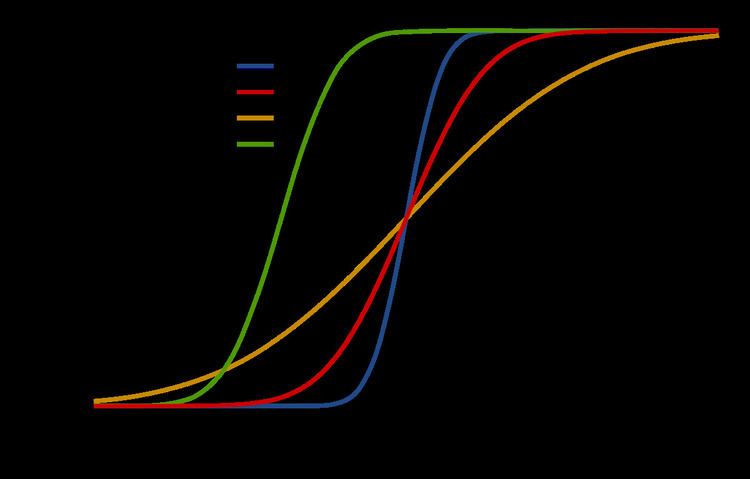
In probability theory and statistics, the cumulative distribution function (CDF) of a real-valued random variable X, or just distribution function of X, evaluated at x, is the probability that X will take a value less than or equal to x.
Contents
- Definition
- Properties
- Examples
- Complementary cumulative distribution function tail distribution
- Folded cumulative distribution
- Inverse distribution function quantile function
- Multivariate case
- Use in statistical analysis
- KolmogorovSmirnov and Kuipers tests
- References
In the case of a continuous distribution, it gives the area under the probability density function from minus infinity to x. Cumulative distribution functions are also used to specify the distribution of multivariate random variables.
Definition
The cumulative distribution function of a real-valued random variable X is the function given by
where the right-hand side represents the probability that the random variable X takes on a value less than or equal to x. The probability that X lies in the semi-closed interval (a, b], where a < b, is therefore
In the definition above, the "less than or equal to" sign, "≤", is a convention, not a universally used one (e.g. Hungarian literature uses "<"), but is important for discrete distributions. The proper use of tables of the binomial and Poisson distributions depends upon this convention. Moreover, important formulas like Paul Lévy's inversion formula for the characteristic function also rely on the "less than or equal" formulation.
If treating several random variables X, Y, ... etc. the corresponding letters are used as subscripts while, if treating only one, the subscript is usually omitted. It is conventional to use a capital F for a cumulative distribution function, in contrast to the lower-case f used for probability density functions and probability mass functions. This applies when discussing general distributions: some specific distributions have their own conventional notation, for example the normal distribution.
The CDF of a continuous random variable X can be expressed as the integral of its probability density function ƒX as follows:
In the case of a random variable X which has distribution having a discrete component at a value b,
If FX is continuous at b, this equals zero and there is no discrete component at b.
Properties
Every cumulative distribution function F is non-decreasing and right-continuous, which makes it a càdlàg function. Furthermore,
Every function with these four properties is a CDF, i.e., for every such function, a random variable can be defined such that the function is the cumulative distribution function of that random variable.
If X is a purely discrete random variable, then it attains values x1, x2, ... with probability pi = P(xi), and the CDF of X will be discontinuous at the points xi and constant in between:
If the CDF F of a real valued random variable X is continuous, then X is a continuous random variable; if furthermore F is absolutely continuous, then there exists a Lebesgue-integrable function f(x) such that
for all real numbers a and b. The function f is equal to the derivative of F almost everywhere, and it is called the probability density function of the distribution of X.
Examples
As an example, suppose
Suppose instead that
Complementary cumulative distribution function (tail distribution)
Sometimes, it is useful to study the opposite question and ask how often the random variable is above a particular level. This is called the complementary cumulative distribution function (ccdf) or simply the tail distribution or exceedance, and is defined as
This has applications in statistical hypothesis testing, for example, because the one-sided p-value is the probability of observing a test statistic at least as extreme as the one observed. Thus, provided that the test statistic, T, has a continuous distribution, the one-sided p-value is simply given by the ccdf: for an observed value t of the test statistic
In survival analysis,
Folded cumulative distribution
While the plot of a cumulative distribution often has an S-like shape, an alternative illustration is the folded cumulative distribution or mountain plot, which folds the top half of the graph over, thus using two scales, one for the upslope and another for the downslope. This form of illustration emphasises the median and dispersion (the mean absolute deviation from the median) of the distribution or of the empirical results.
Inverse distribution function (quantile function)
If the CDF F is strictly increasing and continuous then
Some distributions do not have a unique inverse (for example in the case where
Some useful properties of the inverse cdf (which are also preserved in the definition of the generalized inverse distribution function) are:
-
F − 1 -
F − 1 ( F ( x ) ) ≤ x -
F ( F − 1 ( p ) ) ≥ p -
F − 1 ( p ) ≤ x if and only ify ≤ F ( p ) - If
Y has aU [ 0 , 1 ] distribution thenF − 1 ( Y ) is distributed asF . This is used in random number generation using the inverse transform sampling-method. - If
{ X α } is a collection of independentF -distributed random variables defined on the same sample space, then there exist random variablesY α Y α U [ 0 , 1 ] andF − 1 ( Y α ) = X α α .
The inverse of the cdf can be used to translate results obtained for the uniform distribution to other distributions.
Multivariate case
When dealing simultaneously with more than one random variable the joint cumulative distribution function can also be defined. For example, for a pair of random variables X,Y, the joint CDF
where the right-hand side represents the probability that the random variable X takes on a value less than or equal to x and that Y takes on a value less than or equal to y.
Every multivariate CDF is:
- Monotonically non-decreasing for each of its variables
- Right-continuous for each of its variables.
-
0 ≤ F ( x 1 , . . . , x n ) ≤ 1 -
lim x 1 , . . . , x n → + ∞ F ( x 1 , . . . , x n ) = 1 andlim x i → − ∞ F ( x 1 , . . . , x n ) = 0 , for all i
Use in statistical analysis
The concept of the cumulative distribution function makes an explicit appearance in statistical analysis in two (similar) ways. Cumulative frequency analysis is the analysis of the frequency of occurrence of values of a phenomenon less than a reference value. The empirical distribution function is a formal direct estimate of the cumulative distribution function for which simple statistical properties can be derived and which can form the basis of various statistical hypothesis tests. Such tests can assess whether there is evidence against a sample of data having arisen from a given distribution, or evidence against two samples of data having arisen from the same (unknown) population distribution.
Kolmogorov–Smirnov and Kuiper's tests
The Kolmogorov–Smirnov test is based on cumulative distribution functions and can be used to test to see whether two empirical distributions are different or whether an empirical distribution is different from an ideal distribution. The closely related Kuiper's test is useful if the domain of the distribution is cyclic as in day of the week. For instance Kuiper's test might be used to see if the number of tornadoes varies during the year or if sales of a product vary by day of the week or day of the month.