Real analysis

Construction of the real numbers

The theorems of real analysis rely intimately upon the structure of the real number line. The real number system consists of a set ( R ), together with two operations (+ and •) and an order (<), and is, formally speaking, an ordered quadruple consisting of these objects: ( R , + , ∙ , < ) . There are several ways of formalizing the definition of the real number system. The synthetic approach gives a list of axioms for the real numbers as a complete ordered field. Under the usual axioms of set theory, one can show that these axioms are categorical, in the sense that there is a model for the axioms, and any two such models are isomorphic. Any one of these models must be explicitly constructed, and most of these models are built using the basic properties of the rational number system as an ordered field. These constructions are described in more detail in the main article.

In addition to these algebraic notions, the real numbers, equipped with the absolute value function as a metric (that is, d : R × R → R ≥ 0 , defined by d ( x , y ) = | x − y | ), constitutes the prototypical example of a metric space. Many important theorems in real analysis (e.g., the intermediate value theorem) remain valid when they are restated as statements involving metric spaces. These theorems are frequently topological in nature, and placing them in the more abstract setting of metric spaces (or topological spaces) may lead to proofs that are shorter, more natural, or more elegant.

Order properties of the real numbers

The real numbers have several important lattice-theoretic properties that are absent in the complex numbers. Most importantly, the real numbers form an ordered field, in which addition and multiplication preserve positivity. Moreover, the ordering of the real numbers is total, and the real numbers have the least upper bound property. These order-theoretic properties lead to a number of important results in real analysis, such as the monotone convergence theorem, the intermediate value theorem and the mean value theorem.

However, while the results in real analysis are stated for real numbers, many of these results can be generalized to other mathematical objects. In particular, many ideas in functional analysis and operator theory generalize properties of the real numbers – such generalizations include the theories of Riesz spaces and positive operators. Also, mathematicians consider real and imaginary parts of complex sequences, or by pointwise evaluation of operator sequences.

Sequences

A sequence is a function whose domain is a countable, totally ordered set, usually taken to be the natural numbers or whole numbers. Occasionally, it is also convenient to consider bidirectional sequences indexed by the set of all integers, including negative indices.

Of interest in real analysis, a real-valued sequence, here indexed by the natural numbers, is a map a : N → R ,   n ↦ a n . Each a ( n ) = a n is referred to as a term (or, less commonly, an element) of the sequence. A sequence is rarely denoted explicitly as a function; instead, by convention, it is almost always notated as if it were an ordered ∞-tuple, with individual terms or a general term enclosed in parentheses:

( a n ) = ( a n ) n ∈ N = ( a 1 , a 2 , a 3 , ⋯ ) .

A sequence that tends to a limit (i.e., lim n → ∞ a n exists) is said to be convergent; otherwise it is divergent. (See the section on limits for details) A real-valued sequence ( a n ) is bounded if there exists M ∈ R such that | a n | < M for all n ∈ N . A real-valued sequence ( a n ) is monotonically increasing or decreasing if

a 1 ≤ a 2 ≤ a 3 ≤ … or a 1 ≥ a 2 ≥ a 3 ≥ …

holds, respectively. If either holds, the sequence is said to be monotonic.

Limits and convergence

A limit is the value that a function or sequence "approaches" as the input or index approaches some value. Limits are essential to calculus (and mathematical analysis in general) and are used to define continuity, derivatives, and integrals. In fact, calculus has been defined as the study of limits and limiting processes.

First proposed by Cauchy and made rigorous by Bolzano and Weierstrass, the concept of a limit allowed Newton and Leibniz's calculus to be studied in a logically sound manner, eventually giving rise to analysis as a mathematical discipline. The modern ε-δ definition of the limit of a function of a real variable is given below.

Definition. Let f be a real-valued function defined on E ⊂ R . We say that f ( x ) tends to L as x approaches x 0 , or that the limit of f ( x ) as x approaches x 0 is L if, for any ϵ > 0 , there exists δ > 0 such that for all x ∈ E , 0 < | x − x 0 | < δ implies that | f ( x ) − L | < ϵ . We write this symbolically as

f ( x ) → L     as     x → x 0 , or lim x → x 0 f ( x ) = L .

Intuitively, this definition can be thought of in the following way: We say that f ( x ) → L as x → x 0 , when we can always find a positive number δ , such that given any positive number ϵ (no matter how small), we can guarantee that f ( x ) and L are less than ϵ apart, as long as x (in the domain of f ) is a real number that is less than δ away from x 0 but distinct from x 0 . The purpose of the last stipulation, which corresponds to the condition 0 < | x − x 0 | in the definition, is to ensure that lim x → x 0 f ( x ) = L does not imply anything about the value of f ( x 0 ) itself. Actually, x 0 does not even need to be in the domain of f in order for lim x → x 0 f ( x ) to exist.

In a closely related context, the concept of a limit applies to the behavior of a sequence ( a n ) when n becomes large.

Definition. Let ( a n ) be a real-valued sequence. We say that ( a n ) converges to a if, for any ϵ > 0 , there exists an natural number N such that n ≥ N implies that | a − a n | < ϵ . We write this symbolically as

a n → a     as     n → ∞ , or lim n → ∞ a n = a ;

if ( a n ) fails to converge, we say that ( a n ) diverges.

Sometimes, it is useful to conclude that a sequence converges, even though the value to which it converges is unknown or irrelevant. In these cases, the concept of a Cauchy sequence is useful.

Definition. Let ( a n ) be a real-valued sequence. We say that ( a n ) is a Cauchy sequence if, for any ϵ > 0 , there exists an natural number N such that m , n ≥ N implies that | a m − a n | < ϵ .

It can be shown that a real-valued sequence is Cauchy if and only if it is convergent. This property of the real numbers is expressed by saying that the real numbers endowed with the standard metric, ( R , | ⋅ | ) , is a complete metric space. In a general metric space, however, a Cauchy sequence need not converge.

In addition, for real-valued sequences that are monotonic, it can be shown that the sequence is bounded if and only if it is convergent.

Continuity

A function from the set of real numbers to the real numbers can be represented by a graph in the Cartesian plane; such a function is continuous if, roughly speaking, the graph is a single unbroken curve with no "holes" or "jumps".

There are several ways to make this intuition mathematically rigorous. Several definitions of varying levels of generality can be given. In cases where two or more definitions are applicable, they are readily shown to be equivalent to one another, so the most convenient definition can be used to determine whether a given function is continuous or not. In the first definition given below, f : I → R is a function defined on a non-degenerate interval I of the set of real numbers as its domain. Some possibilities include I = R , the whole set of real numbers, an open interval I = ( a , b ) = { x ∈ R | a < x < b } , or a closed interval I = [ a , b ] = { x ∈ R | a ≤ x ≤ b } . Here, a and b are distinct real numbers, and we exclude the case of I being empty or consisting of only one point, in particular.

Definition. If I ⊂ R is a non-degenerate interval, we say that f : I → R is continuous at p ∈ E if lim x → p f ( x ) = f ( p ) . We say that f is a continuous map if f is continuous at every p ∈ I .

In contrast to the requirements for f to have a limit at a point p , which do not constrain the behavior of f at p itself, the following two conditions, in addition to the existence of lim x → p f ( x ) , must also hold in order for f to be continuous at p : (i) f must be defined at p , i.e., p is in the domain of f ; and (ii) f ( x ) → f ( p ) as x → p . The definition above actually applies to any domain E that does not contain an isolated point, or equivalently, E where every p ∈ E is a limit point of E . A more general definition applying to f : X → R with a general domain X ⊂ R is the following:

Definition. If X is an arbitrary subset of R , we say that f : X → R is continuous at p ∈ X if, for any ϵ > 0 , there exists δ > 0 such that for all x ∈ X , | x − p | < δ implies that | f ( x ) − f ( p ) | < ϵ . We say that f is a continuous map if f is continuous at every p ∈ X .

A consequence of this definition is that f is trivially continuous at any isolated point p ∈ X . This somewhat unintuitive treatment of isolated points is necessary to ensure that our definition of continuity for functions on the real line is consistent with the most general definition of continuity for maps between topological spaces (which includes metric spaces and R in particular as special cases). This definition, which extends beyond the scope of our discussion of real analysis, is given below for completeness.

Definition. If X and Y are topological spaces, we say that f : X → Y is continuous at p ∈ X if f − 1 ( V ) is a neighborhood of p in X for every neighborhood V of f ( p ) in Y . We say that f is a continuous map if f − 1 ( U ) is open in X for every U open in Y .

(Here, f − 1 ( S ) refers to the preimage of S ⊂ Y under f .)

Uniform continuity

Definition. If X is a subset of the real numbers, we say a function f : X → R is uniformly continuous on X if, for any ϵ > 0 , there exists a δ > 0 such that for all x , y ∈ X , | x − y | < δ implies that | f ( x ) − f ( y ) | < ϵ .

Explicitly, when a function is uniformly continuous on X , the choice of δ needed to fulfill the definition must work for all of X for a given ϵ . In contrast, when a function is continuous at every point p ∈ X (or said to be continuous on X ), the choice of δ may depend on both ϵ and p . Importantly, in contrast to simple continuity, uniform continuity is a property of a function that only makes sense with a specified domain; to speak of uniform continuity at a single point p is meaningless.

On a compact set, it is easily shown that all continuous functions are uniformly continuous. If E is a bounded noncompact subset of R , then there exists f : E → R that is continuous but not uniformly continuous. As a simple example, consider f : ( 0 , 1 ) → R defined by f ( x ) = 1 / x . By choosing points close to 0, we can always make | f ( x ) − f ( y ) | > ϵ for any single choice of δ > 0 , for a given ϵ > 0 .

Absolute continuity

Let I ⊂ R be an interval on the real line. A function f : I → R is absolutely continuous on I if for every positive number ϵ , there is a positive number δ such that whenever a finite sequence of pairwise disjoint sub-intervals ( x 1 , y 1 ) , ( x 2 , y 2 ) , … , ( x n , y n ) of I satisfies

∑ k = 1 n ( y k − x k ) < δ

then

∑ k = 1 n | f ( y k ) − f ( x k ) | < ϵ .

Absolutely continuous functions are continuous: consider the case n = 1 in this definition. The collection of all absolutely continuous functions on I is denoted AC(I).

The following conditions on a real-valued function f on a compact interval [a,b] are equivalent:

(1) f is absolutely continuous; (2) f has a derivative f ′ almost everywhere, the derivative is Lebesgue integrable, and f ( x ) = f ( a ) + ∫ a x f ′ ( t ) d t for all x on [a,b]; (3) there exists a Lebesgue integrable function g on [a,b] such that f ( x ) = f ( a ) + ∫ a x g ( t ) d t for all x on [a,b].

If these equivalent conditions are satisfied then necessarily g = f ′ almost everywhere.

Equivalence between (1) and (3) is known as the fundamental theorem of Lebesgue integral calculus, due to Lebesgue.

Series

Given an (infinite) sequence ( a n ) , we can define an associated series as the formal mathematical object a 1 + a 2 + a 3 + ⋯ = ∑ n = 1 ∞ a n , sometimes simply written as ∑ a n . The partial sums of a series ∑ a n are the numbers s n = ∑ j = 1 n a j . A series ∑ a n is said to be convergent if the sequence consisting of its partial sums, ( s n ) , is convergent; otherwise it is divergent. The sum of a convergent series is defined as the number s = lim n → ∞ s n .

It is to be emphasized that the word "sum" is used here in a metaphorical sense as a shorthand for taking the limit of a sequence of partial sums and should not be interpreted as simply "adding" an infinite number of terms. The terms of a series, for instance, cannot be rearranged to give the same sum unless certain conditions are met, unlike what is permitted for a finite sum (see the article on the Riemann rearrangement theorem for further discussion).

An example of a convergent series is a geometric series which forms the basis of one of Zeno's famous paradoxes:

∑ n = 1 ∞ 1 2 n = 1 2 + 1 4 + 1 8 + ⋯ = 1 .

In contrast, the harmonic series has been known since the Middle Ages to be a divergent series:

∑ n = 1 ∞ 1 n = 1 + 1 2 + 1 3 + ⋯ = ∞ .

(Here, " = ∞ " is merely a notational convention to indicate that the partial sums of the series grow without bound.)

A series ∑ a n is said to converge absolutely if ∑ | a n | is convergent. A convergent series ∑ a n for which ∑ | a n | diverges is said to converge conditionally (or nonabsolutely). It is easily shown that absolute convergence of a series implies its convergence. On the other hand, an example of a conditionally convergent series is

∑ n = 1 ∞ ( − 1 ) n − 1 n = 1 − 1 2 + 1 3 − 1 4 + ⋯ = log ⁡ 2 .

Taylor series

The Taylor series of a real or complex-valued function ƒ(x) that is infinitely differentiable at a real or complex number a is the power series

f ( a ) + f ′ ( a ) 1 ! ( x − a ) + f ″ ( a ) 2 ! ( x − a ) 2 + f ( 3 ) ( a ) 3 ! ( x − a ) 3 + ⋯ .

which can be written in the more compact sigma notation as

∑ n = 0 ∞ f ( n ) ( a ) n ! ( x − a ) n

where n! denotes the factorial of n and ƒ ⁽ⁿ⁾(a) denotes the nth derivative of ƒ evaluated at the point a. The derivative of order zero ƒ is defined to be ƒ itself and (x − a)⁰ and 0! are both defined to be 1. In the case that a = 0, the series is also called a Maclaurin series.

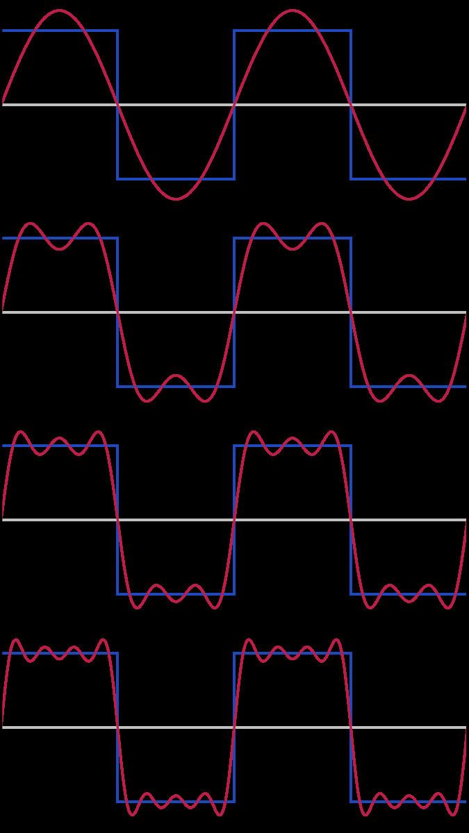
Fourier series

A Fourier series decomposes periodic functions or periodic signals into the sum of a (possibly infinite) set of simple oscillating functions, namely sines and cosines (or complex exponentials). The study of Fourier series is a branch of Fourier analysis.

Differentiation

Formally, the derivative of the function f at a is the limit

f ′ ( a ) = lim h → 0 f ( a + h ) − f ( a ) h

If the derivative exists everywhere, the function is differentiable. One can take higher derivatives as well, by iterating this process.

One can classify functions by their differentiability class. The class C⁰ consists of all continuous functions. The class C¹ consists of all differentiable functions whose derivative is continuous; such functions are called continuously differentiable. Thus, a C¹ function is exactly a function whose derivative exists and is of class C⁰. In general, the classes C^k can be defined recursively by declaring C⁰ to be the set of all continuous functions and declaring C^k for any positive integer k to be the set of all differentiable functions whose derivative is in C^k−1. In particular, C^k is contained in C^k−1 for every k, and there are examples to show that this containment is strict. C^∞ is the intersection of the sets C^k as k varies over the non-negative integers. C^ω consists of all analytic functions, and is strictly contained in C^∞.

Riemann integration

The Riemann integral is defined in terms of Riemann sums of functions with respect to tagged partitions of an interval. Let [a,b] be a closed interval of the real line; then a tagged partition of [a,b] is a finite sequence

a = x 0 ≤ t 1 ≤ x 1 ≤ t 2 ≤ x 2 ≤ ⋯ ≤ x n − 1 ≤ t n ≤ x n = b .

This partitions the interval [a,b] into n sub-intervals [x_i−1, x_i] indexed by i, each of which is "tagged" with a distinguished point t_i ∈ [x_i−1, x_i]. A Riemann sum of a function f with respect to such a tagged partition is defined as

∑ i = 1 n f ( t i ) Δ i ;

thus each term of the sum is the area of a rectangle with height equal to the function value at the distinguished point of the given sub-interval, and width the same as the sub-interval width. Let Δ_i = x_i−x_i−1 be the width of sub-interval i; then the mesh of such a tagged partition is the width of the largest sub-interval formed by the partition, max_i=1...n Δ_i. The Riemann integral of a function f over the interval [a,b] is equal to S if:

For all ε > 0 there exists δ > 0 such that, for any tagged partition [a,b] with mesh less than δ, we have | S − ∑ i = 1 n f ( t i ) Δ i | < ε .

When the chosen tags give the maximum (respectively, minimum) value of each interval, the Riemann sum becomes an upper (respectively, lower) Darboux sum, suggesting the close connection between the Riemann integral and the Darboux integral.

Lebesgue integration

Lebesgue integration is a mathematical construction that extends the integral to a larger class of functions; it also extends the domains on which these functions can be defined.

Distributions

Distributions (or generalized functions) are objects that generalize functions. Distributions make it possible to differentiate functions whose derivatives do not exist in the classical sense. In particular, any locally integrable function has a distributional derivative.

Relation to complex analysis

Real analysis is an area of analysis that studies concepts such as sequences and their limits, continuity, differentiation, integration and sequences of functions. By definition, real analysis focuses on the real numbers, often including positive and negative infinity to form the extended real line. Real analysis is closely related to complex analysis, which studies broadly the same properties of complex numbers. In complex analysis, it is natural to define differentiation via holomorphic functions, which have a number of useful properties, such as repeated differentiability, expressability as power series, and satisfying the Cauchy integral formula.

In real analysis, it is usually more natural to consider differentiable, smooth, or harmonic functions, which are more widely applicable, but may lack some more powerful properties of holomorphic functions. However, results such as the fundamental theorem of algebra are simpler when expressed in terms of complex numbers.

Techniques from the theory of analytic functions of a complex variable are often used in real analysis – such as evaluation of real integrals by residue calculus.

Important results

Important results include the Bolzano–Weierstrass and Heine–Borel theorems, the intermediate value theorem and mean value theorem, the fundamental theorem of calculus, and the monotone convergence theorem.

Various ideas from real analysis can be generalized from real space to general metric spaces, as well as to measure spaces, Banach spaces, and Hilbert spaces.