Limit of a function

History

Although implicit in the development of calculus of the 17th and 18th centuries, the modern idea of the limit of a function goes back to Bolzano who, in 1817, introduced the basics of the epsilon-delta technique to define continuous functions. However, his work was not known during his lifetime (Felscher 2000). Cauchy discussed variable quantities, infinitesimals, and limits and defined continuity of y = f ( x ) by saying that an infinitesimal change in x necessarily produces an infinitesimal change in y in his 1821 book Cours d'analyse, while (Grabiner 1983) claims that he only gave a verbal definition. Weierstrass first introduced the epsilon-delta definition of limit in the form it is usually written today. He also introduced the notations lim and lim_x→x0 (Burton 1997).

The modern notation of placing the arrow below the limit symbol is due to Hardy in his book A Course of Pure Mathematics in 1908 (Miller 2004).

Motivation

Imagine a person walking over a landscape represented by the graph of y = f(x). Her horizontal position is measured by the value of x, much like the position given by a map of the land or by a global positioning system. Her altitude is given by the coordinate y. She is walking towards the horizontal position given by x = p. As she gets closer and closer to it, she notices that her altitude approaches L. If asked about the altitude of x = p, she would then answer L.

What, then, does it mean to say that her altitude approaches L? It means that her altitude gets nearer and nearer to L except for a possible small error in accuracy. For example, suppose we set a particular accuracy goal for our traveler: she must get within ten meters of L. She reports back that indeed she can get within ten meters of L, since she notes that when she is within fifty horizontal meters of p, her altitude is always ten meters or less from L.

The accuracy goal is then changed: can she get within one vertical meter? Yes. If she is anywhere within seven horizontal meters of p, then her altitude always remains within one meter from the target L. In summary, to say that the traveler's altitude approaches L as her horizontal position approaches p means that for every target accuracy goal, however small it may be, there is some neighborhood of p whose altitude fulfills that accuracy goal.

The initial informal statement can now be explicated:

The limit of a function f(x) as x approaches p is a number L with the following property: given any target distance from L, there is a distance from p within which the values of f(x) remain within the target distance.

This explicit statement is quite close to the formal definition of the limit of a function with values in a topological space.

To say that

lim x → p f ( x ) = L ,

means that ƒ(x) can be made as close as desired to L by making x close enough, but not equal, to p.

The following definitions (known as (ε, δ)-definitions) are the generally accepted ones for the limit of a function in various contexts.

Functions of a single variable

Suppose f : R → R is defined on the real line and p,L ∈ R. It is said the limit of f, as x approaches p, is L and written

lim x → p f ( x ) = L ,  

if the following property holds:

For every real ε > 0, there exists a real δ > 0 such that for all real x, 0 < | x − p | < δ implies | f(x) − L | < ε.

The value of the limit does not depend on the value of f(p), nor even that p be in the domain of f.

A more general definition applies for functions defined on subsets of the real line. Let (a, b) be an open interval in R, and p a point of (a, b). Let f be a real-valued function defined on all of (a, b) except possibly at p itself. It is then said that the limit of f, as x approaches p, is L if, for every real ε > 0, there exists a real δ > 0 such that 0 < | x − p | < δ and x ∈ (a, b) implies | f(x) − L | < ε.

Here again the limit does not depend on f(p) being well-defined.

The letters ε and δ can be understood as "error" and "distance", and in fact Cauchy used ε as an abbreviation for "error" in some of his work (Grabiner 1983), though in his definition of continuity he used an infinitesimal α rather than either ε or δ (see Cours d'Analyse). In these terms, the error (ε) in the measurement of the value at the limit can be made as small as desired by reducing the distance (δ) to the limit point. As discussed below this definition also works for functions in a more general context. The idea that δ and ε represent distances helps suggest these generalizations.

Existence and one-sided limits

Alternatively x may approach p from above (right) or below (left), in which case the limits may be written as

lim x → p + f ( x ) = L

or

lim x → p − f ( x ) = L

respectively. If these limits exist at p and are equal there, then this can be referred to as the limit of f(x) at p. If the one-sided limits exist at p, but are unequal, there is no limit at p (the limit at p does not exist). If either one-sided limit does not exist at p, the limit at p does not exist.

A formal definition is as follows. The limit of f(x) as x approaches p from above is L if, for every ε > 0, there exists a δ > 0 such that |f(x) − L| < ε whenever 0 < x − p < δ. The limit of f(x) as x approaches p from below is L if, for every ε > 0, there exists a δ > 0 such that |f(x) − L| < ε whenever 0 < p − x < δ.

If the limit does not exist then the oscillation of f at p is non-zero.

More general subsets

Apart from open intervals, limits can be defined for functions on arbitrary subsets of R, as follows. Let f be a real-valued function defined on a subset S of the real line. Let p be a limit point of S—that is, p is the limit of some sequence of distinct elements of S. The limit of f, as x approaches p from values in S, is L if, for every ε > 0, there exists a δ > 0 such that 0 < | x − p | < δ and x ∈ S implies | f(x) − L | < ε.

This limit is often written

L = lim x → p x ∈ S f ( x ) .

The condition that f be defined on S is that S be a subset of the domain of f. This generalization includes as special cases limits on an interval, as well as left-handed limits of real-valued functions (e.g., by taking S to be an open interval of the form ( − ∞ , a ) ), and right-handed limits (e.g., by taking S to be an open interval of the form ( a , ∞ ) ).

Deleted versus non-deleted limits

The definition of limit given here does not depend on how (or whether) f is defined at p. Bartle (1967), refers to this as a deleted limit, because it excludes the value of f at p. The corresponding non-deleted limit does depend on the value of f at p, if p is in the domain of f:

A number L is the non-deleted limit of f as x approaches p if, for every ε > 0, there exists a δ > 0 such that | x − p | < δ and x ∈ Dm(f) implies | f(x) − L | < ε.

The definition is the same, except that the neighborhood | x − p | < δ now includes the point p, in contrast to the (deleted) neighborhood 0 < | x − p | < δ. Bartle (1967) notes that although by "limit" some authors do mean this non-deleted limit, deleted limits are the most popular. For example, Apostol (1974), Courant (1924), Hardy (1921), Rudin (1964), Whittaker & Watson (1902) all by "limit" mean the deleted version.

Non-existence of one-sided limit(s)

The function

f ( x ) = { sin ⁡ 5 x − 1  for  x < 1 0  for  x = 1 0.1 x − 1  for  x > 1

has no limit at x 0 = 1 (the left-hand limit does not exist due to the oscillatory nature of the sine function, and the right-hand limit does not exist due to the asymptotic behaviour of the reciprocal function), but has a limit at every other x-coordinate.

The function

f ( x ) = { 1 x  rational  0 x  irrational 

(the Dirichlet function) has no limit at any x-coordinate.

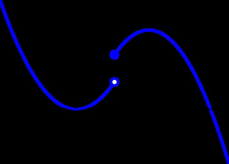
Non-equality of one-sided limits

The function

f ( x ) = { 1  for  x < 0 2  for  x ≥ 0

has a limit at every non-zero x-coordinate (the limit equals 1 for negative x and equals 2 for positive x). The limit at x = 0 does not exist (the left-hand limit equals 1, whereas the right-hand limit equals 2).

Limits at only one point

The functions

f ( x ) = { x x  rational  0 x  irrational 

and

f ( x ) = { | x | x  rational  0 x  irrational 

both have a limit at x = 0 and it equals 0.

Limits at countably many points

The function

f ( x ) = { sin ⁡ x x  irrational  1 x  rational 

has a limit at any x-coordinate of the form π 2 + 2 n π , where n is any integer.

Functions on metric spaces

Suppose M and N are subsets of metric spaces A and B, respectively, and f : M → N is defined between M and N, with x ∈ M, p a limit point of M and L ∈ N. It is said that the limit of f as x approaches p is L and write

lim x → p f ( x ) = L

if the following property holds:

For every ε > 0, there exists a δ > 0 such that d_B(f(x), L) < ε whenever 0 < d_A(x, p) < δ.

Again, note that p need not be in the domain of f, nor does L need to be in the range of f, and even if f(p) is defined it need not be equal to L.

An alternative definition using the concept of neighbourhood is as follows:

lim x → p f ( x ) = L

if, for every neighbourhood V of L in B, there exists a neighbourhood U of p in A such that f(U ∩ M − {p}) ⊆ V.

Functions on topological spaces

Suppose X,Y are topological spaces with Y a Hausdorff space. Let p be a limit point of Ω ⊆ X, and L ∈Y. For a function f : Ω → Y, it is said that the limit of f as x approaches p is L (i.e., f(x) → L as x → p) and written

lim x → p f ( x ) = L

if the following property holds:

For every open neighborhood V of L, there exists an open neighborhood U of p such that f(U ∩ Ω − {p}) ⊆ V.

This last part of the definition can also be phrased "there exists an open punctured neighbourhood U of p such that f(U∩Ω) ⊆ V ".

Note that the domain of f does not need to contain p. If it does, then the value of f at p is irrelevant to the definition of the limit. In particular, if the domain of f is X − {p} (or all of X), then the limit of f as x → p exists and is equal to L if, for all subsets Ω of X with limit point p, the limit of the restriction of f to Ω exists and is equal to L. Sometimes this criterion is used to establish the non-existence of the two-sided limit of a function on R by showing that the one-sided limits either fail to exist or do not agree. Such a view is fundamental in the field of general topology, where limits and continuity at a point are defined in terms of special families of subsets, called filters, or generalized sequences known as nets.

Alternatively, the requirement that Y be a Hausdorff space can be relaxed to the assumption that Y be a general topological space, but then the limit of a function may not be unique. In particular, one can no longer talk about the limit of a function at a point, but rather a limit or the set of limits at a point.

A function is continuous in a limit point p of and in its domain if and only if f(p) is the (or, in the general case, a) limit of f(x) as x tends to p.

Limits at infinity

For f(x) a real function, the limit of f as x approaches infinity is L, denoted

lim x → ∞ f ( x ) = L ,

means that for all ε > 0 , there exists c such that | f ( x ) − L | < ε whenever x > c. Or, symbolically:

∀ ε > 0 ∃ c ∀ x > c : | f ( x ) − L | < ε

Similarly, the limit of f as x approaches negative infinity is L, denoted

lim x → − ∞ f ( x ) = L ,

means that for all ε > 0 there exists c such that | f ( x ) − L | < ε whenever x < c. Or, symbolically:

∀ ε > 0 ∃ c ∀ x < c : | f ( x ) − L | < ε

For example

lim x → − ∞ e x = 0.

Infinite limits

Limits can also have infinite values. When infinities are not considered legitimate values, which is standard (but see below), a formalist will insist upon various circumlocutions. For example, rather than say that a limit is infinity, the proper thing is to say that the function "diverges" or "grows without bound". In particular, the following informal example of how to pronounce the notation is arguably inappropriate in the classroom (or any other formal setting). In any case, for example the limit of f as x approaches a is infinity, denoted

lim x → a f ( x ) = ∞ ,

means that for all ε > 0 there exists δ > 0 such that f ( x ) > ε whenever | x − a | < δ .

These ideas can be combined in a natural way to produce definitions for different combinations, such as

lim x → ∞ f ( x ) = ∞ , lim x → a + f ( x ) = − ∞ .

For example

lim x → 0 + ln ⁡ x = − ∞ .

Limits involving infinity are connected with the concept of asymptotes.

These notions of a limit attempt to provide a metric space interpretation to limits at infinity. However, note that these notions of a limit are consistent with the topological space definition of limit if

a neighborhood of −∞ is defined to contain an interval [−∞, c) for some c ∈ R

a neighborhood of ∞ is defined to contain an interval (c, ∞] where c ∈ R

a neighborhood of a∈R is defined in the normal way metric space R

In this case, R is a topological space and any function of the form f: X → Y with X, Y⊆ R is subject to the topological definition of a limit. Note that with this topological definition, it is easy to define infinite limits at finite points, which have not been defined above in the metric sense.

Alternative notation

Many authors allow for the projectively extended real line to be used as a way to include infinite values as well as extended real line. With this notation, the extended real line is given as R ∪ {−∞, +∞} and the projectively extended real line is R ∪ {∞} where a neighborhood of ∞ is a set of the form {x: | x | > c}. The advantage is that one only needs three definitions for limits (left, right, and central) to cover all the cases. As presented above, for a completely rigorous account, we would need to consider 15 separate cases for each combination of infinities (five directions: −∞, left, central, right, and +∞; three bounds: −∞, finite, or +∞). There are also noteworthy pitfalls. For example, when working with the extended real line, x − 1 does not possess a central limit (which is normal):

lim x → 0 + 1 x = + ∞ , lim x → 0 − 1 x = − ∞ .

In contrast, when working with the projective real line, infinities (much like 0) are unsigned, so, the central limit does exist in that context:

lim x → 0 + 1 x = lim x → 0 − 1 x = lim x → 0 1 x = ∞ .

In fact there are a plethora of conflicting formal systems in use. In certain applications of numerical differentiation and integration, it is, for example, convenient to have signed zeroes. A simple reason has to do with the converse of lim x → 0 − x − 1 = − ∞ , namely, it is convenient for lim x → − ∞ x − 1 = − 0 to be considered true. Such zeroes can be seen as an approximation to infinitesimals.

Limits at infinity for rational functions

There are three basic rules for evaluating limits at infinity for a rational function f(x) = p(x)/q(x): (where p and q are polynomials):

If the degree of p is greater than the degree of q, then the limit is positive or negative infinity depending on the signs of the leading coefficients;

If the degree of p and q are equal, the limit is the leading coefficient of p divided by the leading coefficient of q;

If the degree of p is less than the degree of q, the limit is 0.

If the limit at infinity exists, it represents a horizontal asymptote at y = L. Polynomials do not have horizontal asymptotes; such asymptotes may however occur with rational functions.

Functions of more than one variable

By noting that |x − p| represents a distance, the definition of a limit can be extended to functions of more than one variable. In the case of a function f : R² → R,

lim ( x , y ) → ( p , q ) f ( x , y ) = L

if

for every ε > 0 there exists a δ > 0 such that for all (x,y) with 0 < ||(x,y) − (p,q)|| < δ, then |f(x,y) − L| < ε

where ||(x,y) − (p,q)|| represents the Euclidean distance. This can be extended to any number of variables.

Sequential limits

Let f : X → Y be a mapping from a topological space X into a Hausdorff space Y, p ∈ X and L ∈ Y.

The sequential limit of f as x tends to p is L if, for every sequence (x_n) in X − {p} that converges to p, the sequence f(x_n) converges to L.

If L is the limit (in the sense above) of f as x approaches p, then it is a sequential limit as well, however the converse need not hold in general. If in addition X is metrizable, then L is the sequential limit of f as x approaches p if and only if it is the limit (in the sense above) of f as x approaches p.

In terms of sequences

For functions on the real line, one way to define the limit of a function is in terms of the limit of sequences. (This definition is usually attributed to Eduard Heine.) In this setting:

lim x → a f ( x ) = L

if and only if for all sequences x n (with x n not equal to a for all n) converging to a the sequence f ( x n ) converges to L . It was shown by Sierpiński in 1916 that proving the equivalence of this definition and the definition above, requires and is equivalent to a weak form of the axiom of choice. Note that defining what it means for a sequence x n to converge to a requires the epsilon, delta method.

Similarly as it was the case of Weierstrass's definition, a more general Heine definition applies to functions defined on subsets of the real line. Let f be a real-valued function with the domain Dm(f). Let a be the limit of a sequence of elements of Dm(f). Then the limit (in this sense) of f is L as x approaches p if for every sequence x n  ∈ Dm(f)  {a} (so that for all n, x n is not equal to a) that converges to a, the sequence f ( x n ) converges to L . This is the same as the definition of a sequential limit in the preceding section obtained by regarding the subset Dm(f) of R as a metric space with the induced metric.

In non-standard calculus

In non-standard calculus the limit of a function is defined by:

lim x → a f ( x ) = L

if and only if for all x ∈ R ∗ , f ∗ ( x ) − L is infinitesimal whenever x − a is infinitesimal. Here R ∗ are the hyperreal numbers and f ∗ is the natural extension of f to the non-standard real numbers. Keisler proved that such a hyperreal definition of limit reduces the quantifier complexity by two quantifiers. On the other hand, Hrbacek writes that for the definitions to be valid for all hyperreal numbers they must implicitly be grounded in the ε-δ method, and claims that, from the pedagogical point of view, the hope that non-standard calculus could be done without ε-δ methods cannot be realized in full. Bŀaszczyk et al. detail the usefulness of microcontinuity in developing a transparent definition of uniform continuity, and characterize Hrbacek's criticism as a "dubious lament".

In terms of nearness

At the 1908 international congress of mathematics F. Riesz introduced an alternate way defining limits and continuity in concept called "nearness". A point x is defined to be near a set A ⊆ R if for every r > 0 there is a point a ∈ A so that | x − a | < r . In this setting the

lim x → a f ( x ) = L

if and only if for all A ⊆ R , L is near f ( A ) whenever a is near A . Here f ( A ) is the set { f ( x ) | x ∈ A } . This definition can also be extended to metric and topological spaces.

Relationship to continuity

The notion of the limit of a function is very closely related to the concept of continuity. A function ƒ is said to be continuous at c if it is both defined at c and its value at c equals the limit of f as x approaches c:

lim x → c f ( x ) = f ( c ) .

(We have here assumed that c is a limit point of the domain of f.)

Properties

If a function f is real-valued, then the limit of f at p is L if and only if both the right-handed limit and left-handed limit of f at p exist and are equal to L.

The function f is continuous at p if and only if the limit of f(x) as x approaches p exists and is equal to f(p). If f : M → N is a function between metric spaces M and N, then it is equivalent that f transforms every sequence in M which converges towards p into a sequence in N which converges towards f(p).

If N is a normed vector space, then the limit operation is linear in the following sense: if the limit of f(x) as x approaches p is L and the limit of g(x) as x approaches p is P, then the limit of f(x) + g(x) as x approaches p is L + P. If a is a scalar from the base field, then the limit of af(x) as x approaches p is aL.

If f is a real-valued (or complex-valued) function, then taking the limit is compatible with the algebraic operations, provided the limits on the right sides of the equations below exist (the last identity only holds if the denominator is non-zero). This fact is often called the algebraic limit theorem.

lim x → p ( f ( x ) + g ( x ) ) = lim x → p f ( x ) + lim x → p g ( x ) lim x → p ( f ( x ) − g ( x ) ) = lim x → p f ( x ) − lim x → p g ( x ) lim x → p ( f ( x ) ⋅ g ( x ) ) = lim x → p f ( x ) ⋅ lim x → p g ( x ) lim x → p ( f ( x ) / g ( x ) ) = lim x → p f ( x ) / lim x → p g ( x )

In each case above, when the limits on the right do not exist, or, in the last case, when the limits in both the numerator and the denominator are zero, nonetheless the limit on the left, called an indeterminate form, may still exist—this depends on the functions f and g. These rules are also valid for one-sided limits, for the case p = ±∞, and also for infinite limits using the rules

q + ∞ = ∞ for q ≠ −∞

q × ∞ = ∞ if q > 0

q × ∞ = −∞ if q < 0

q / ∞ = 0 if q ≠ ± ∞

(see extended real number line).

Note that there is no general rule for the case q / 0; it all depends on the way 0 is approached. Indeterminate forms—for instance, 0/0, 0×∞, ∞−∞, and ∞/∞—are also not covered by these rules, but the corresponding limits can often be determined with L'Hôpital's rule or the Squeeze theorem.

Limits of compositions of functions

In general, from knowing that

lim y → b f ( y ) = c and lim x → a g ( x ) = b ,

it does not follow that lim x → a f ( g ( x ) ) = c . However, this "chain rule" does hold if one of the following additional conditions holds:

f(b) = c (that is, f is continuous at b), or

g does not take the value b near a (that is, there exists a δ > 0 such that if 0 < | x − a | < δ then | g ( x ) − b | > 0 ).

As an example of this phenomenon, consider the following functions that violates both additional restrictions:

f ( x ) = g ( x ) = { 0 if  x ≠ 0 1 if  x = 0 .

Since the value at f(0) is a removable discontinuity,

lim x → a f ( x ) = 0 for all a .

Thus, the naïve chain rule would suggest that the limit of f(f(x)) is 0. However, it is the case that

f ( f ( x ) ) = { 1 if  x ≠ 0 0 if  x = 0

and so

lim x → a f ( f ( x ) ) = 1 for all a .

Rational functions

For n a nonnegative integer and constants a 1 , a 2 , a 3 , … , a n and b 1 , b 2 , b 3 , … , b n ,

lim x → ∞ a 1 x n + a 2 x n − 1 + a 3 x n − 2 + . . . + a n b 1 x n + b 2 x n − 1 + b 3 x n − 2 + . . . + b n = a 1 b 1

This can be proven by dividing both the numerator and denominator by x n . If the numerator is a polynomial of higher degree, the limit does not exist. If the denominator is of higher degree, the limit is 0.

Trigonometric functions

lim x → 0 sin ⁡ x x = 1

lim x → 0 1 − cos ⁡ x x = 0

lim x → ∞ x sin ⁡ ( 1 x ) = 1

Exponential functions

lim x → 0 ( 1 + x ) 1 x = lim r → ∞ ( 1 + 1 r ) r = e

lim x → 0 e x − 1 x = 1

lim x → 0 e a x − 1 b x = a b

lim x → 0 c a x − 1 b x = a b ln ⁡ c

Logarithmic functions

lim x → 0 ln ⁡ ( 1 + x ) x = 1

lim x → 0 ln ⁡ ( 1 + a x ) b x = a b

lim x → 0 log c ⁡ ( 1 + a x ) b x = a b ln ⁡ c

L'Hôpital's rule

This rule uses derivatives to find limits of indeterminate forms 0/0 or ±∞/∞, and only applies to such cases. Other indeterminate forms may be manipulated into this form. Given two functions f(x) and g(x), defined over an open interval I containing the desired limit point c, then if:

1. lim x → c f ( x ) = lim x → c g ( x ) = 0 , or lim x → c f ( x ) = ± lim x → c g ( x ) = ± ∞ , and
2. f and g are differentiable over I ∖ { c } , and
3. g ′ ( x ) ≠ 0 for all x ∈ I ∖ { c } , and
4. lim x → c f ′ ( x ) g ′ ( x ) exists,

then:

lim x → c f ( x ) g ( x ) = lim x → c f ′ ( x ) g ′ ( x )

Normally, the first condition is the most important one.

For example: lim x → 0 sin ⁡ ( 2 x ) sin ⁡ ( 3 x ) = lim x → 0 2 cos ⁡ ( 2 x ) 3 cos ⁡ ( 3 x ) = 2 ⋅ 1 3 ⋅ 1 = 2 3 .

Summations and integrals

Specifying an infinite bound on a summation or integral is a common shorthand for specifying a limit.

A short way to write the limit lim n → ∞ ∑ i = s n f ( i ) is ∑ i = s ∞ f ( i ) .

A short way to write the limit lim x → ∞ ∫ a x f ( t ) d t is ∫ a ∞ f ( t ) d t .

A short way to write the limit lim x → − ∞ ∫ x b f ( t ) d t is ∫ − ∞ b f ( t ) d t .