Factorial

Definition

The factorial function is formally defined by the product

n ! = ∏ k = 1 n k ,

or by the recurrence relation

n ! = { 1 if  n = 0 , ( n − 1 ) ! × n if  n > 0.

The factorial function can also be defined by using the power rule as

n ! = D n x n .

All of the above definitions incorporate the instance

0 ! = 1 ,  

in the first case by the convention that the product of no numbers at all is 1. This is convenient because:

There is exactly one permutation of zero objects (with nothing to permute, "everything" is left in place).

The recurrence relation (n + 1)! = n! × (n + 1), valid for n > 0, extends to n = 0.

It allows for the expression of many formulae, such as the exponential function, as a power series:

It makes many identities in combinatorics valid for all applicable sizes. The number of ways to choose 0 elements from the empty set is ( 0 0 ) = 0 ! 0 ! 0 ! = 1 . More generally, the number of ways to choose (all) n elements among a set of n is ( n n ) = n ! n ! 0 ! = 1 .

The factorial function can also be defined for non-integer values using more advanced mathematics, detailed in the section below. This more generalized definition is used by advanced calculators and mathematical software such as Maple or Mathematica.

Applications

Although the factorial function has its roots in combinatorics, formulas involving factorials occur in many areas of mathematics.

There are n! different ways of arranging n distinct objects into a sequence, the permutations of those objects.

Often factorials appear in the denominator of a formula to account for the fact that ordering is to be ignored. A classical example is counting k-combinations (subsets of k elements) from a set with n elements. One can obtain such a combination by choosing a k-permutation: successively selecting and removing an element of the set, k times, for a total of

possibilities. This however produces the k-combinations in a particular order that one wishes to ignore; since each k-combination is obtained in k! different ways, the correct number of k-combinations is n k _ k ! = n ( n − 1 ) ( n − 2 ) ⋯ ( n − k + 1 ) k ( k − 1 ) ( k − 2 ) ⋯ 1 . This number is known as the binomial coefficient ( n k ) , because it is also the coefficient of X^k in (1 + X)ⁿ.

Factorials occur in algebra for various reasons, such as via the already mentioned coefficients of the binomial formula, or through averaging over permutations for symmetrization of certain operations.

Factorials also turn up in calculus; for example they occur in the denominators of the terms of Taylor's formula, where they are used as compensation terms due to the n-th derivative of xⁿ being equivalent to n!.

Factorials are also used extensively in probability theory.

Factorials can be useful to facilitate expression manipulation. For instance the number of k-permutations of n can be written as

while this is inefficient as a means to compute that number, it may serve to prove a symmetry property of binomial coefficients:

Rate of growth and approximations for large n

As n grows, the factorial n! increases faster than all polynomials and exponential functions (but slower than double exponential functions) in n.

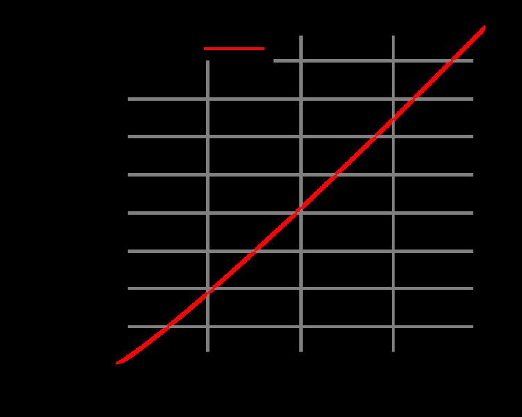
Most approximations for n! are based on approximating its natural logarithm

ln ⁡ n ! = ∑ x = 1 n ln ⁡ x .

The graph of the function f(n) = ln n! is shown in the figure on the right. It looks approximately linear for all reasonable values of n, but this intuition is false. We get one of the simplest approximations for ln n! by bounding the sum with an integral from above and below as follows:

∫ 1 n ln ⁡ x d x ≤ ∑ x = 1 n ln ⁡ x ≤ ∫ 0 n ln ⁡ ( x + 1 ) d x

which gives us the estimate

n ln ⁡ ( n e ) + 1 ≤ ln ⁡ n ! ≤ ( n + 1 ) ln ⁡ ( n + 1 e ) + 1.

Hence ln ⁡ n ! ∼ n ln ⁡ n (see Big O notation). This result plays a key role in the analysis of the computational complexity of sorting algorithms (see comparison sort). From the bounds on ln n! deduced above we get that

e ( n e ) n ≤ n ! ≤ e ( n + 1 e ) n + 1 .

It is sometimes practical to use weaker but simpler estimates. Using the above formula it is easily shown that for all n we have ( n / 3 ) n < n ! , and for all n ≥ 6 we have n ! < ( n / 2 ) n .

For large n we get a better estimate for the number n! using Stirling's approximation:

n ! ∼ 2 π n ( n e ) n .

This in fact comes from an asymptotic series for the logarithm, and n factorial lies between this and the next approximation:

2 π n ( n e ) n < n ! < 2 π n ( n e ) n e 1 12 n .

Another approximation for ln n! is given by Srinivasa Ramanujan (Ramanujan 1988)

ln ⁡ n ! ≈ n ln ⁡ n − n + ln ⁡ ( n ( 1 + 4 n ( 1 + 2 n ) ) ) 6 + ln ⁡ ( π ) 2

or

n ! ≈ 2 π n ( n e ) n [ 1 + 1 / ( 2 n ) + 1 / ( 8 n 2 ) ] 1 / 6 .

Both this and 2 π n ( n e ) n e 1 12 n give a relative error on the order of 1/n³, but Ramanujan's is about four times more accurate. However, if we use two correction terms (as in Ramanujan's approximation) the relative error will be of order 1/n⁵:

n ! ≈ 2 π n ( n e ) n exp ⁡ ( 1 12 n − 1 360 n 3 )

Computation

If efficiency is not a concern, computing factorials is trivial from an algorithmic point of view: successively multiplying a variable initialized to 1 by the integers 2 up to n (if any) will compute n!, provided the result fits in the variable. In functional languages, the recursive definition is often implemented directly to illustrate recursive functions.

The main practical difficulty in computing factorials is the size of the result. To assure that the exact result will fit for all legal values of even the smallest commonly used integral type (8-bit signed integers) would require more than 700 bits, so no reasonable specification of a factorial function using fixed-size types can avoid questions of overflow. The values 12! and 20! are the largest factorials that can be stored in, respectively, the 32-bit and 64-bit integers commonly used in personal computers. Floating-point representation of an approximated result allows going a bit further, but this also remains quite limited by possible overflow. Most calculators use scientific notation with 2-digit decimal exponents, and the largest factorial that fits is then 69!, because 69! < 10¹⁰⁰ < 70!. Other implementations (e.g., computer software such as spreadsheet programs) can often handle larger values.

Most software applications will compute small factorials by direct multiplication or table lookup. Larger factorial values can be approximated using Stirling's formula. Wolfram Alpha can calculate exact results for the ceiling function and floor function applied to the binary, natural and common logarithm of n! for values of n up to 249999, and up to 20,000,000! for the integers.

If the exact values of large factorials are needed, they can be computed using arbitrary-precision arithmetic. Instead of doing the sequential multiplications ( ( 1 × 2 ) × 3 ) × 4 × ⋯ , a program can partition the sequence into two parts, whose products are roughly the same size, and multiply them using a divide-and-conquer method. This is often more efficient.

The asymptotically best efficiency is obtained by computing n! from its prime factorization. As documented by Peter Borwein, prime factorization allows n! to be computed in time O(n(log n log log n)²), provided that a fast multiplication algorithm is used (for example, the Schönhage–Strassen algorithm). Peter Luschny presents source code and benchmarks for several efficient factorial algorithms, with or without the use of a prime sieve.

Number theory

Factorials have many applications in number theory. In particular, n! is necessarily divisible by all prime numbers up to and including n. As a consequence, n > 5 is a composite number if and only if

( n − 1 ) !   ≡   0 ( mod n ) .

A stronger result is Wilson's theorem, which states that

( p − 1 ) !   ≡   − 1 ( mod p )

if and only if p is prime.

Legendre's formula gives the multiplicity of the prime p occurring in the prime factorization of n ! as

∑ i = 1 ∞ ⌊ n p i ⌋

or, equivalently,

n − s p ( n ) p − 1 ,

where s p ( n ) denotes the sum of the standard base-p digits of n.

Adding 1 to a factorial n! yields a number that is divisible by a prime larger than n. This fact can be used to prove Euclid's theorem that the number of primes is infinite. Primes of the form n! ± 1 are called factorial primes.

Series of reciprocals

The reciprocals of factorials produce a convergent series whose sum is Euler's number e:

∑ n = 0 ∞ 1 n ! = 1 1 + 1 1 + 1 2 + 1 6 + 1 24 + 1 120 + ⋯ = e .

Although the sum of this series is an irrational number, it is possible to multiply the factorials by positive integers to produce a convergent series with a rational sum:

∑ n = 0 ∞ 1 ( n + 2 ) n ! = 1 2 + 1 3 + 1 8 + 1 30 + 1 144 + ⋯ = 1 .

The convergence of this series to 1 can be seen from the fact that its partial sums are less than one by an inverse factorial. Therefore, the factorials do not form an irrationality sequence.

The Gamma and Pi functions

Besides nonnegative integers, the factorial function can also be defined for non-integer values, but this requires more advanced tools from mathematical analysis. One function that "fills in" the values of the factorial (but with a shift of 1 in the argument) is called the Gamma function, denoted Γ(z), defined for all complex numbers z except the non-positive integers, and given when the real part of z is positive by

Γ ( z ) = ∫ 0 ∞ t z − 1 e − t d t .

Its relation to the factorials is that for any natural number n

n ! = Γ ( n + 1 ) .

Euler's original formula for the Gamma function was

Γ ( z ) = lim n → ∞ n z n ! ∏ k = 0 n ( z + k ) .

An alternative notation, originally introduced by Gauss, is sometimes used. The Pi function, denoted Π(z) for real numbers z no less than 0, is defined by

Π ( z ) = ∫ 0 ∞ t z e − t d t .

In terms of the Gamma function it is

Π ( z ) = Γ ( z + 1 ) .

It truly extends the factorial in that

Π ( n ) = n !  for  n ∈ N .

In addition to this, the Pi function satisfies the same recurrence as factorials do, but at every complex value z where it is defined

Π ( z ) = z Π ( z − 1 ) .

In fact, this is no longer a recurrence relation but a functional equation. Expressed in terms of the Gamma function this functional equation takes the form

Γ ( n + 1 ) = n Γ ( n ) .

Since the factorial is extended by the Pi function, for every complex value z where it is defined, we can write:

z ! = Π ( z )

The values of these functions at half-integer values is therefore determined by a single one of them; one has

Γ ( 1 2 ) = ( − 1 2 ) ! = Π ( − 1 2 ) = π ,

from which it follows that for n ∈ N,

Γ ( 1 2 + n ) = ( − 1 2 + n ) ! = Π ( − 1 2 + n ) = π ∏ k = 1 n 2 k − 1 2 = ( 2 n ) ! 4 n n ! π = ( 2 n − 1 ) ! 2 2 n − 1 ( n − 1 ) ! π .

For example,

Γ ( 4.5 ) = 3.5 ! = Π ( 3.5 ) = 1 2 ⋅ 3 2 ⋅ 5 2 ⋅ 7 2 π = 8 ! 4 4 4 ! π = 7 ! 2 7 3 ! π = 105 16 π ≈ 11.63.

It also follows that for n ∈ N,

Γ ( 1 2 − n ) = ( − 1 2 − n ) ! = Π ( − 1 2 − n ) = π ∏ k = 1 n 2 1 − 2 k = ( − 4 ) n n ! ( 2 n ) ! π .

For example,

Γ ( − 2.5 ) = ( − 3.5 ) ! = Π ( − 3.5 ) = 2 − 1 ⋅ 2 − 3 ⋅ 2 − 5 π = ( − 4 ) 3 3 ! 6 ! π = − 8 15 π ≈ − 0.9453.

The Pi function is certainly not the only way to extend factorials to a function defined at almost all complex values, and not even the only one that is analytic wherever it is defined. Nonetheless it is usually considered the most natural way to extend the values of the factorials to a complex function. For instance, the Bohr–Mollerup theorem states that the Gamma function is the only function that takes the value 1 at 1, satisfies the functional equation Γ(n + 1) = nΓ(n), is meromorphic on the complex numbers, and is log-convex on the positive real axis. A similar statement holds for the Pi function as well, using the Π(n) = nΠ(n − 1) functional equation.

However, there exist complex functions that are probably simpler in the sense of analytic function theory and which interpolate the factorial values. For example, Hadamard's 'Gamma'-function (Hadamard 1894) which, unlike the Gamma function, is an entire function.

Euler also developed a convergent product approximation for the non-integer factorials, which can be seen to be equivalent to the formula for the Gamma function above:

n ! = Π ( n ) = ∏ k = 1 ∞ ( k + 1 k ) n k n + k = [ ( 2 1 ) n 1 n + 1 ] [ ( 3 2 ) n 2 n + 2 ] [ ( 4 3 ) n 3 n + 3 ] ⋯ .

However, this formula does not provide a practical means of computing the Pi or Gamma function, as its rate of convergence is slow.

Applications of the Gamma function

The volume of an n-dimensional hypersphere of radius R is

V n = π n / 2 Γ ( ( n / 2 ) + 1 ) R n .

Factorial at the complex plane

Representation through the Gamma-function allows evaluation of factorial of complex argument. Equilines of amplitude and phase of factorial are shown in figure. Let   f = ρ exp ⁡ ( i φ ) = ( x + i y ) ! = Γ ( x + i y + 1 ) . Several levels of constant modulus (amplitude) ρ = c o n s t and constant phase φ = c o n s t are shown. The grid covers range   − 3 ≤ x ≤ 3   ,   − 2 ≤ y ≤ 2   with unit step. The scratched line shows the level φ = ± π .

Thin lines show intermediate levels of constant modulus and constant phase. At poles x + i y ∈ ( n e g a t i v e   i n t e g e r s ) , phase and amplitude are not defined. Equilines are dense in vicinity of singularities along negative integer values of the argument.

For | z | < 1 , the Taylor expansions can be used:

z ! = ∑ n = 0 ∞ g n z n .

The first coefficients of this expansion are

where γ is the Euler constant and ζ is the Riemann zeta function. Computer algebra systems such as SageMath can generate many terms of this expansion.

Approximations of factorial

For the large values of the argument, factorial can be approximated through the integral of the digamma function, using the continued fraction representation. This approach is due to T. J. Stieltjes (1894). Writing z! = exp(P(z)) where P(z) is

P ( z ) = p ( z ) + log ⁡ ( 2 π ) / 2 − z + ( z + 1 2 ) log ⁡ ( z ) ,

Stieltjes gave a continued fraction for p(z)

p ( z ) = a 0 z + a 1 z + a 2 z + a 3 z + ⋱

The first few coefficients a_n are

There is a misconception that log ⁡ ( z ! ) = P ( z ) or log ⁡ ( Γ ( z + 1 ) ) = P ( z ) for any complex z ≠ 0. Indeed, the relation through the logarithm is valid only for specific range of values of z in vicinity of the real axis, while | ℑ ( Γ ( z + 1 ) ) | < π . The larger is the real part of the argument, the smaller should be the imaginary part. However, the inverse relation, z! = exp(P(z)), is valid for the whole complex plane apart from zero. The convergence is poor in vicinity of the negative part of the real axis. (It is difficult to have good convergence of any approximation in vicinity of the singularities). While | ℑ ( z ) | > 2 or ℜ ( z ) > 2 , the 6 coefficients above are sufficient for the evaluation of the factorial with the complex<double> precision. For higher precision more coefficients can be computed by a rational QD-scheme (H. Rutishauser's QD algorithm).

Non-extendability to negative integers

The relation n! = n × (n − 1)! allows one to compute the factorial for an integer given the factorial for a smaller integer. The relation can be inverted so that one can compute the factorial for an integer given the factorial for a larger integer:

( n − 1 ) ! = n ! n .

Note, however, that this recursion does not permit us to compute the factorial of a negative integer; use of the formula to compute (−1)! would require a division by zero, and thus blocks us from computing a factorial value for every negative integer. (Similarly, the Gamma function is not defined for non-positive integers, though it is defined for all other complex numbers.)

Factorial-like products and functions

There are several other integer sequences similar to the factorial that are used in mathematics:

Double factorial

The product of all the odd integers up to some odd positive integer n is called the double factorial of n, and denoted by n!!. That is,

( 2 k − 1 ) ! ! = ∏ i = 1 k ( 2 i − 1 ) = ( 2 k ) ! 2 k k ! = 2 k P k 2 k = ( 2 k ) k _ 2 k .

For example, 9!! = 1 × 3 × 5 × 7 × 9 = 945.

The sequence of double factorials for n = 1, 3, 5, 7, ... starts as

1, 3, 15, 105, 945, 10395, 135135, .... (sequence A001147 in the OEIS)

Double factorial notation may be used to simplify the expression of certain trigonometric integrals, to provide an expression for the values of the Gamma function at half-integer arguments and the volume of hyperspheres, and to solve many counting problems in combinatorics including counting binary trees with labeled leaves and perfect matchings in complete graphs.

Multifactorials

A common related notation is to use multiple exclamation points to denote a multifactorial, the product of integers in steps of two ( n ! ! ), three ( n ! ! ! ), or more. The double factorial is the most commonly used variant, but one can similarly define the triple factorial ( n ! ! ! ) and so on. One can define the k-th factorial, denoted by n ! ( k ) , recursively for positive integers as

n ! ( k ) = { n if  0 < n ≤ k n ( ( n − k ) ! ( k ) ) if  n > k

though see the alternative definition below. In addition, similarly to 0! = 1!/1 = 1, one can define:

n ! ( k ) = 1   if  − k < n ≤ 0

Some mathematicians have suggested an alternative notation of n ! 2 for the double factorial and similarly n ! k for other multifactorials, but this has not come into general use.

In the same way that n ! is not defined for negative integers, and n ! ! is not defined for negative even integers, n ! ( k ) is not defined for negative integers divisible by k .

Alternative extension of the multifactorial

Alternatively, the multifactorial z!^(k) can be extended to most real and complex numbers z by noting that when z is one more than a positive multiple of k then

z ! ( k ) = z ( z − k ) ⋯ ( k + 1 ) = k ( z − 1 ) / k ( z k ) ( z − k k ) ⋯ ( k + 1 k ) = k ( z − 1 ) / k Γ ( z k + 1 ) Γ ( 1 k + 1 ) .

This last expression is defined much more broadly than the original; with this definition, z!^(k) is defined for all complex numbers except the negative real numbers divisible by k. This definition is consistent with the earlier definition only for those integers z satisfying z ≡ 1 mod k.

In addition to extending z!^(k) to most complex numbers z, this definition has the feature of working for all positive real values of k. Furthermore, when k = 1, this definition is mathematically equivalent to the Π(z) function, described above. Also, when k = 2, this definition is mathematically equivalent to the alternative extension of the double factorial.

Generalized Stirling numbers expanding the multifactorial functions

A class of generalized Stirling numbers of the first kind is defined for α > 0 by the following triangular recurrence relation:

[ n k ] α = ( α n + 1 − 2 α ) [ n − 1 k ] α + [ n − 1 k − 1 ] α + δ n , 0 δ k , 0 .

These generalized α -factorial coefficients then generate the distinct symbolic polynomial products defining the multiple factorial, or α -factorial functions, ( x − 1 ) ! ( α ) , as

( x − 1 | α ) n _ := ∏ i = 0 n − 1 ( x − 1 − i α ) = ( x − 1 ) ( x − 1 − α ) ⋯ ( x − 1 − ( n − 1 ) α ) = ∑ k = 0 n [ n k ] ( − α ) n − k ( x − 1 ) k = ∑ k = 1 n [ n k ] α ( − 1 ) n − k x k − 1 .

Notice that the distinct polynomial expansions in the previous equations actually define the α -factorial products for multiple distinct cases of the least residues x ≡ n 0 ( mod α ) for n 0 ∈ { 0 , 1 , 2 , … , α − 1 } .

The generalized α -factorial polynomials, σ n ( α ) ( x ) where σ n ( 1 ) ( x ) ≡ σ n ( x ) , which generalize the Stirling (convolution) polynomials from the single factorial case to the multifactorial cases, are defined by

σ n ( α ) ( x ) := [ x x − n ] ( α ) ( x − n − 1 ) ! x !

for 0 ≤ n ≤ x . These polynomials have a particularly nice closed-form ordinary generating function given by

∑ n ≥ 0 x ⋅ σ n ( α ) ( x ) z n = e ( 1 − α ) z ( α z e α z e α z − 1 ) x .

Other combinatorial properties and expansions of these generalized α -factorial triangles and polynomial sequences are considered in .

Exact finite sums involving the multiple factorial functions

Suppose that n ≥ 1 and α ≥ 2 are integer-valued. Then we can expand the next single finite sums involving the multifactorial, or α -factorial functions, ( α n − 1 ) ! ( α ) , in terms of the Pochhammer symbol and the generalized, rational-valued binomial coefficients as

( α n − 1 ) ! ( α ) = ∑ k = 0 n − 1 ( n − 1 k + 1 ) ( − 1 ) k × ( 1 α ) − ( k + 1 ) ( 1 α − n ) k + 1 × ( α ( k + 1 ) − 1 ) ! ( α ) ( α ( n − k − 1 ) − 1 ) ! ( α ) = ∑ k = 0 n − 1 ( n − 1 k + 1 ) ( − 1 ) k × ( 1 α + k − n k + 1 ) ( 1 α − 1 k + 1 ) × ( α ( k + 1 ) − 1 ) ! ( α ) ( α ( n − k − 1 ) − 1 ) ! ( α ) ,

and moreover, we similarly have double sum expansions of these functions given by

( α n − 1 ) ! ( α ) = ∑ k = 0 n − 1 ∑ i = 0 k + 1 ( n − 1 k + 1 ) ( k + 1 i ) ( − 1 ) k α k + 1 − i ( α i − 1 ) ! ( α ) ( α ( n − 1 − k ) − 1 ) ! ( α ) × ( n − 1 − k ) k + 1 − i = ∑ k = 0 n − 1 ∑ i = 0 k + 1 ( n − 1 k + 1 ) ( k + 1 i ) ( n − 1 − i k + 1 − i ) ( − 1 ) k α k + 1 − i ( α i − 1 ) ! ( α ) ( α ( n − 1 − k ) − 1 ) ! ( α ) × ( k + 1 − i ) ! .

We notice that the first two sums above are similar in form to a known non-round combinatorial identity for the double factorial function when α := 2 given by

( 2 n − 1 ) ! ! = ∑ k = 0 n − 1 ( n k + 1 ) ( 2 k − 1 ) ! ! ( 2 n − 2 k − 3 ) ! ! .

Additional finite sum expansions of congruences for the α -factorial functions, ( α n − d ) ! ( α ) , modulo any prescribed integer h ≥ 2 for any 0 ≤ d < α are found in .

Primorial

The primorial (sequence A002110 in the OEIS) is similar to the factorial, but with the product taken only over the prime numbers.

Quadruple factorial

Contrary to consistency with the above definition of the term double factorial, the quadruple factorial is not the multifactorial n!⁽⁴⁾; it is a much larger number given by (2n)!/n!, starting as

1, 2, 12, 120, 1680, 30240, 665280, ... (sequence A001813 in the OEIS).

It is also equal to

2 n ( 2 n ) ! n ! 2 n = 2 n ( 2 ⋅ 4 ⋯ 2 n ) ( 1 ⋅ 3 ⋯ ( 2 n − 1 ) ) 2 ⋅ 4 ⋯ 2 n = ( 1 ⋅ 2 ) ⋅ ( 3 ⋅ 2 ) ⋯ ( ( 2 n − 1 ) ⋅ 2 ) = ( 4 n − 2 ) ! ( 4 ) .

Superfactorial

Neil Sloane and Simon Plouffe defined a superfactorial in The Encyclopedia of Integer Sequences (Academic Press, 1995) to be the product of the first n factorials. So the superfactorial of 4 is

sf ⁡ ( 4 ) = 1 ! × 2 ! × 3 ! × 4 ! = 288.

In general

sf ⁡ ( n ) = ∏ k = 1 n k ! = ∏ k = 1 n k n − k + 1 = 1 n ⋅ 2 n − 1 ⋅ 3 n − 2 ⋯ ( n − 1 ) 2 ⋅ n 1 .

Equivalently, the superfactorial is given by the formula

sf ⁡ ( n ) = ∏ 0 ≤ i < j ≤ n ( j − i )

which is the determinant of a Vandermonde matrix.

The sequence of superfactorials starts (from n = 0 ) as

1, 1, 2, 12, 288, 34560, 24883200, 125411328000, ... (sequence A000178 in the OEIS)

Alternative definition

Clifford Pickover in his 1995 book Keys to Infinity used a new notation, n$, to define the superfactorial

n $ ≡ n ! n ! ⋅ ⋅ ⋅ n ! ⏟ n ! ,

or as,

n $ = n ! [ 4 ] n !

where the [4] notation denotes the hyper4 operator, or using Knuth's up-arrow notation,

n $ = ( n ! ) ↑↑ ( n ! ) .

This sequence of superfactorials starts:

1 $ = 1 2 $ = 2 2 = 4 3 $ = 6 [ 4 ] 6 = 6 6 = 6 6 6 6 6 6 .

Here, as is usual for compound exponentiation, the grouping is understood to be from right to left:

a b c = a ( b c ) .

Hyperfactorial

Occasionally the hyperfactorial of n is considered. It is written as H(n) and defined by

H ( n ) = ∏ k = 1 n k k = 1 1 ⋅ 2 2 ⋅ 3 3 ⋯ ( n − 1 ) n − 1 ⋅ n n .

For n = 1, 2, 3, 4, ... the values H(n) are 1, 4, 108, 27648,... (sequence A002109 in the OEIS).

The asymptotic growth rate is

H ( n ) ∼ A n ( 6 n 2 + 6 n + 1 ) / 12 e − n 2 / 4

where A = 1.2824... is the Glaisher–Kinkelin constant. H(14) = 1.8474...×10⁹⁹ is already almost equal to a googol, and H(15) = 8.0896...×10¹¹⁶ is almost of the same magnitude as the Shannon number, the theoretical number of possible chess games. Compared to the Pickover definition of the superfactorial, the hyperfactorial grows relatively slowly.

The hyperfactorial function can be generalized to complex numbers in a similar way as the factorial function. The resulting function is called the K-function.