
 | ||
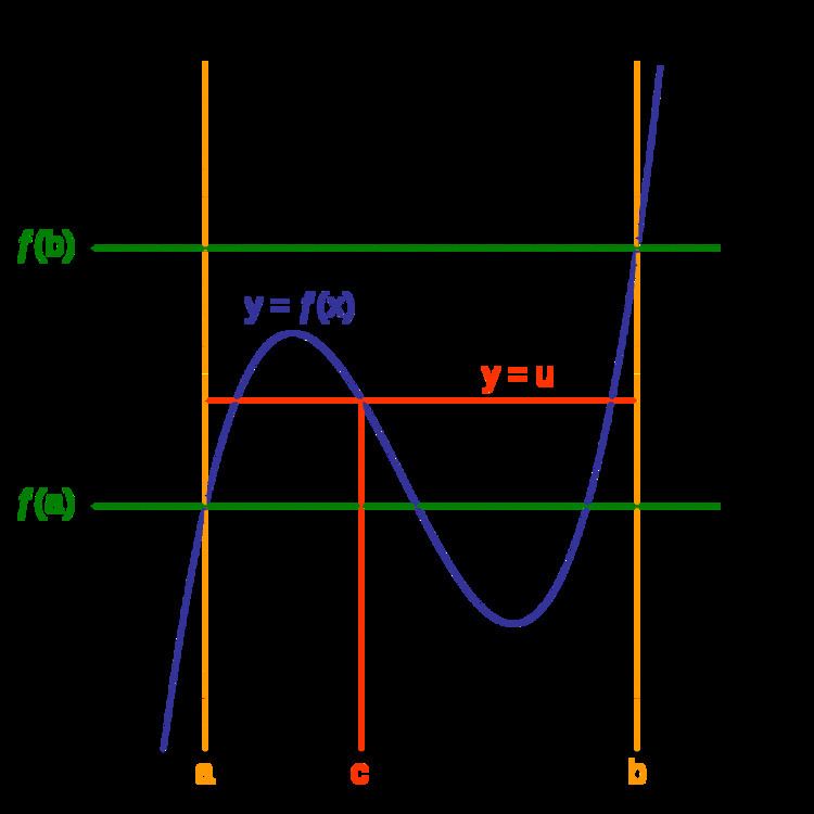
In mathematical analysis, the intermediate value theorem states that if a continuous function, f, with an interval, [a, b], as its domain, takes values f(a) and f(b) at each end of the interval, then it also takes any value between f(a) and f(b) at some point within the interval.
Contents
- Motivation
- Theorem
- Relation to completeness
- Proof
- History
- Generalizations
- Converse is false
- Practical applications
- References
This has two important corollaries: 1) If a continuous function has values of opposite sign inside an interval, then it has a root in that interval (Bolzano's theorem). 2) The image of a continuous function over an interval is itself an interval.
Motivation
This captures an intuitive property of continuous functions: given f continuous on [1, 2] with the known values f(1) = 3 and f(2) = 5. Then the graph of y = f(x) must pass through the horizontal line y = 4 while x moves from 1 to 2. It represents the idea that the graph of a continuous function on a closed interval can be drawn without lifting your pencil from the paper.
Theorem
The intermediate value theorem states the following.
Consider an interval
Remark: Version II states that the set of function values has no gap. For any two function values
A subset of the real numbers with no internal gap is an interval. Version I is obviously contained in Version II.
Relation to completeness
The theorem depends on, and is equivalent to, the completeness of the real numbers. The intermediate value theorem does not apply to the rational numbers ℚ because gaps exists between rational numbers; irrational numbers fill those gaps. For example, the function
Proof
The theorem may be proved as a consequence of the completeness property of the real numbers as follows:
We shall prove the first case,
Let
Fix some
for all
Choose
Both inequalities
are valid for all
The intermediate value theorem is an easy consequence of the basic properties of connected sets: the preservation of connectedness under continuous functions and the characterization of connected subsets of ℝ as intervals (see below for details and alternate proof). The latter characterization is ultimately a consequence of the least-upper-bound property of the real numbers.
The intermediate value theorem can also be proved using the methods of non-standard analysis, which places "intuitive" arguments involving infinitesimals on a rigorous footing. (See the article: non-standard calculus.)
History
For u = 0 above, the statement is also known as Bolzano's theorem. This theorem was first proved by Bernard Bolzano in 1817. Augustin-Louis Cauchy provided a proof in 1821. Both were inspired by the goal of formalizing the analysis of functions and the work of Joseph-Louis Lagrange. The idea that continuous functions possess the intermediate value property has an earlier origin. Simon Stevin proved the intermediate value theorem for polynomials (using a cubic as an example) by providing an algorithm for constructing the decimal expansion of the solution. The algorithm iteratively subdivides the interval into 10 parts, producing an additional decimal digit at each step of the iteration. Before the formal definition of continuity was given, the intermediate value property was given as part of the definition of a continuous function. Proponents include Louis Arbogast, who assumed the functions to have no jumps, satisfy the intermediate value property and have increments whose sizes corresponded to the sizes of the increments of the variable. Earlier authors held the result to be intuitively obvious and requiring no proof. The insight of Bolzano and Cauchy was to define a general notion of continuity (in terms of infinitesimals in Cauchy's case and using real inequalities in Bolzano's case), and to provide a proof based on such definitions.
Generalizations
The intermediate value theorem is closely linked to the topological notion of connectedness and follows from the basic properties of connected sets in metric spaces and connected subsets of ℝ in particular:
In fact, connectedness is a topological property and (*) generalizes to topological spaces: If
Recall the first version of the intermediate value theorem, stated previously:
Intermediate value theorem. (Version I). Consider a closed interval
The intermediate value theorem is an immediate consequence of these two properties of connectedness:
Proof: By (**),
The intermediate value theorem generalizes in a natural way: Suppose that X is a connected topological space and (Y, <) is a totally ordered set equipped with the order topology, and let f : X → Y be a continuous map. If a and b are two points in X and u is a point in Y lying between f(a) and f(b) with respect to <, then there exists c in X such that f(c) = u. The original theorem is recovered by noting that ℝ is connected and that its natural topology is the order topology.
The Brouwer fixed-point theorem is a related theorem that, in one dimension gives a special case of the intermediate value theorem.
Converse is false
A "Darboux function" is a real-valued function f that has the "intermediate value property", i.e., that satisfies the conclusion of the intermediate value theorem: for any two values a and b in the domain of f, and any y between f(a) and f(b), there is some c between a and b with f(c) = y. The intermediate value theorem says that every continuous function is a Darboux function. However, not every Darboux function is continuous; i.e., the converse of the intermediate value theorem is false.
As an example, take the function f : [0, ∞) → [−1, 1] defined by f(x) = sin(1/x) for x > 0 and f(0) = 0. This function is not continuous at x = 0 because the limit of f(x) as x tends to 0 does not exist; yet the function has the intermediate value property. Another, more complicated example is given by the Conway base 13 function.
Historically, this intermediate value property has been suggested as a definition for continuity of real-valued functions; this definition was not adopted.
Darboux's theorem states that all functions that result from the differentiation of some other function on some interval have the intermediate value property (even though they need not be continuous).
Practical applications
The theorem implies that on any great circle around the world, for the temperature, pressure, elevation, carbon dioxide concentration, or any other similar scalar quantity which varies continuously, there will always exist two antipodal points that share the same value for that variable.
Proof: Take f to be any continuous function on a circle. Draw a line through the center of the circle, intersecting it at two opposite points A and B. Let d be defined by the difference f(A) − f(B). If the line is rotated 180 degrees, the value −d will be obtained instead. Due to the intermediate value theorem there must be some intermediate rotation angle for which d = 0, and as a consequence f(A) = f(B) at this angle.
This is a special case of a more general result called the Borsuk–Ulam theorem.
Another generalization for which this holds is for any closed convex n (n > 1) dimensional shape. Specifically, for any continuous function whose domain is the given shape, and any point inside the shape (not necessarily its center), there exist two antipodal points with respect to the given point whose functional value is the same. The proof is identical to the one given above.
The theorem also underpins the explanation of why rotating a wobbly table will bring it to stability (subject to certain easily met constraints).