
 | ||
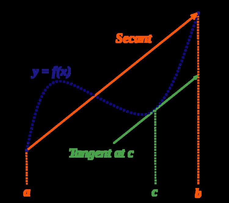
In mathematics, the mean value theorem states, roughly, that for a given a planar arc between two endpoints, there is at least one point at which the tangent to the arc is parallel to the secant through its endpoints.
Contents
- History
- Formal statement
- Proof
- A simple application
- Cauchys mean value theorem
- Proof of Cauchys mean value theorem
- Generalization for determinants
- Mean value theorem in several variables
- Mean value theorem for vector valued functions
- First mean value theorem for definite integrals
- Proof of the first mean value theorem for definite integrals
- Second mean value theorem for definite integrals
- Mean value theorem for integration fails for vector valued functions
- A probabilistic analogue of the mean value theorem
- Generalization in complex analysis
- References
This theorem is used to prove statements about a function on an interval starting from local hypotheses about derivatives at points of the interval.
More precisely, if a function
It is one of the most important results in real analysis.
History
A special case of this theorem was first described by Parameshvara (1370–1460), from the Kerala school of astronomy and mathematics in India, in his commentaries on Govindasvāmi and Bhaskara II. A restricted form of the theorem was proved by Rolle in 1691; the result was what is now known as Rolle's theorem, and was proved only for polynomials, without the techniques of calculus. The mean value theorem in its modern form was stated and proved by Cauchy in 1823.
Formal statement
Let
The mean value theorem is a generalization of Rolle's theorem, which assumes
The mean value theorem is still valid in a slightly more general setting. One only needs to assume that
exists as a finite number or equals
Note that the theorem, as stated, is false if a differentiable function is complex-valued instead of real-valued. For example, define
while
Proof
The expression
Define
By Rolle's theorem, since
as required.
A simple application
Assume that f is a continuous, real-valued function, defined on an arbitrary interval I of the real line. If the derivative of f at every interior point of the interval I exists and is zero, then f is constant in the interior.
Proof: Assume the derivative of f at every interior point of the interval I exists and is zero. Let (a, b) be an arbitrary open interval in I. By the mean value theorem, there exists a point c in (a,b) such that
This implies that f(a) = f(b). Thus, f is constant on the interior of I and thus is constant on I by continuity. (See below for a multivariable version of this result.)
Remarks:
Cauchy's mean value theorem
Cauchy's mean value theorem, also known as the extended mean value theorem, is a generalization of the mean value theorem. It states: If functions f and g are both continuous on the closed interval [a, b], and differentiable on the open interval (a, b), then there exists some c ∈ (a, b), such that
Of course, if g(a) ≠ g(b) and if g′(c) ≠ 0, this is equivalent to:
Geometrically, this means that there is some tangent to the graph of the curve
which is parallel to the line defined by the points (f(a), g(a)) and (f(b), g(b)). However Cauchy's theorem does not claim the existence of such a tangent in all cases where (f(a), g(a)) and (f(b), g(b)) are distinct points, since it might be satisfied only for some value c with f′(c) = g′(c) = 0, in other words a value for which the mentioned curve is stationary; in such points no tangent to the curve is likely to be defined at all. An example of this situation is the curve given by
which on the interval [−1, 1] goes from the point (−1, 0) to (1, 0), yet never has a horizontal tangent; however it has a stationary point (in fact a cusp) at t = 0.
Cauchy's mean value theorem can be used to prove l'Hôpital's rule. The mean value theorem is the special case of Cauchy's mean value theorem when g(t) = t.
Proof of Cauchy's mean value theorem
The proof of Cauchy's mean value theorem is based on the same idea as the proof of the mean value theorem.
Generalization for determinants
Assume that
There exists
Notice that
and if we place
The proof of the generalization is quite simple: each of
Mean value theorem in several variables
The mean value theorem generalizes to real functions of multiple variables. The trick is to use parametrization to create a real function of one variable, and then apply the one-variable theorem.
Let
for some
where
In particular, when the partial derivatives of
As an application of the above, we prove that
for every
The above arguments are made in a coordinate-free manner; hence, they generalize to the case when
Mean value theorem for vector-valued functions
There is no exact analog of the mean value theorem for vector-valued functions.
In Principles of Mathematical Analysis, Rudin gives an inequality which can be applied to many of the same situations to which the mean value theorem is applicable in the one dimensional case:
Theorem. For a continuous vector-valued function
Jean Dieudonné in his classic treatise Foundations of Modern Analysis discards the mean value theorem and replaces it by mean inequality as the proof is not constructive and one cannot find the mean value and in applications one only needs mean inequality. Serge Lang in Analysis I uses the mean value theorem, in integral form, as an instant reflex but this use requires the continuity of the derivative. If one uses the Henstock–Kurzweil integral one can have the mean value theorem in integral form without the additional assumption that derivative should be continuous as every derivative is Henstock–Kurzweil integrable. The problem is roughly speaking the following: If f : U → Rm is a differentiable function (where U ⊂ Rn is open) and if x + th, x, h ∈ Rn, t ∈ [0, 1] is the line segment in question (lying inside U), then one can apply the above parametrization procedure to each of the component functions fi (i = 1, ..., m) of f (in the above notation set y = x + h). In doing so one finds points x + tih on the line segment satisfying
But generally there will not be a single point x + t*h on the line segment satisfying
for all i simultaneously. For example, define:
Then
However a certain type of generalization of the mean value theorem to vector-valued functions is obtained as follows: Let f be a continuously differentiable real-valued function defined on an open interval I, and let x as well as x + h be points of I. The mean value theorem in one variable tells us that there exists some t* between 0 and 1 such that
On the other hand, we have, by the fundamental theorem of calculus followed by a change of variables,
Thus, the value f′(x + t*h) at the particular point t* has been replaced by the mean value
This last version can be generalized to vector valued functions:
Lemma 1. Let U ⊂ Rn be open, f : U → Rm continuously differentiable, and x ∈ U, h ∈ Rn vectors such that the line segment x + th, 0 ≤ t ≤ 1 remains in U. Then we have:Proof. Let f1, ..., fm denote the components of f and define:
Then we have
The claim follows since Df is the matrix consisting of the components
Proof. Let u in Rm denote the value of the integral
Now we have (using the Cauchy–Schwarz inequality):
Now cancelling the norm of u from both ends gives us the desired inequality.
Mean Value Inequality. If the norm of Df(x + th) is bounded by some constant M for t in [0, 1], thenProof. From Lemma 1 and 2 it follows that
First mean value theorem for definite integrals
Let f : [a, b] → R be a continuous function. Then there exists c in (a, b) such that
Since the mean value of f on [a, b] is defined as
we can interpret the conclusion as f achieves its mean value at some c in (a, b).
In general, if f : [a, b] → R is continuous and g is an integrable function that does not change sign on [a, b], then there exists c in (a, b) such that
Proof of the first mean value theorem for definite integrals
Suppose f : [a, b] → R is continuous and g is a nonnegative integrable function on [a, b]. By the extreme value theorem, there exists m and M such that for each x in [a, b],
Now let
If
means
so for any c in (a, b),
If I ≠ 0, then
By the intermediate value theorem, f attains every value of the interval [m, M], so for some c in [a, b]
that is,
Finally, if g is negative on [a, b], then
and we still get the same result as above.
QED
Second mean value theorem for definite integrals
There are various slightly different theorems called the second mean value theorem for definite integrals. A commonly found version is as follows:
If G : [a, b] → R is a positive monotonically decreasing function and φ : [a, b] → R is an integrable function, then there exists a number x in (a, b] such thatHere
Mean value theorem for integration fails for vector-valued functions
If the function
For example, consider the following 2-dimensional function defined on an
Then, by symmetry it is easy to see that the mean value of
However, there is no point in which
A probabilistic analogue of the mean value theorem
Let X and Y be non-negative random variables such that E[X] < E[Y] < ∞ and
Let g be a measurable and differentiable function such that E[g(X)], E[g(Y)] < ∞, and let its derivative g′ be measurable and Riemann-integrable on the interval [x, y] for all y ≥ x ≥ 0. Then, E[g′(Z)] is finite and
Generalization in complex analysis
As noted above, the theorem does not hold for differentiable complex-valued functions. Instead, a generalization of the theorem is stated such:
Let f : Ω → C be a holomorphic function on the open convex set Ω, and let a and b be distinct points in Ω. Then there exist points u, v on Lab (the line segment from a to b) such that
Where Re() is the Real part and Im() is the Imaginary part of a complex-valued function.