
 | ||
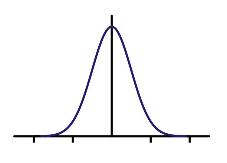
In electronics and signal processing, a Gaussian filter is a filter whose impulse response is a Gaussian function (or an approximation to it). Gaussian filters have the properties of having no overshoot to a step function input while minimizing the rise and fall time. This behavior is closely connected to the fact that the Gaussian filter has the minimum possible group delay. It is considered the ideal time domain filter, just as the sinc is the ideal frequency domain filter. These properties are important in areas such as oscilloscopes and digital telecommunication systems.
Contents
Mathematically, a Gaussian filter modifies the input signal by convolution with a Gaussian function; this transformation is also known as the Weierstrass transform.
Definition
The one-dimensional Gaussian filter has an impulse response given by
and the frequency response is given by the Fourier transform
with
and the frequency response is given by
By writing
where the standard deviations are expressed in their physical units, e.g. in the case of time and frequency in seconds and Hertz.
In two dimensions, it is the product of two such Gaussians, one per direction:
where x is the distance from the origin in the horizontal axis, y is the distance from the origin in the vertical axis, and σ is the standard deviation of the Gaussian distribution.
Digital implementation
The Gaussian function is for
Filtering involves convolution. The filter function is said to be the kernel of an integral transform. The Gaussian kernel is continuous. Most commonly, the discrete equivalent is the sampled Gaussian kernel that is produced by sampling points from the continuous Gaussian. An alternate method is to use the discrete Gaussian kernel which has superior characteristics for some purposes. Unlike the sampled Gaussian kernel, the discrete Gaussian kernel is the solution to the discrete diffusion equation.
Since the Fourier transform of the Gaussian function yields a Gaussian function, the signal (preferably after being divided into overlapping windowed blocks) can be transformed with a Fast Fourier transform, multiplied with a Gaussian function and transformed back. This is the standard procedure of applying an arbitrary finite impulse response filter, with the only difference that the Fourier transform of the filter window is explicitly known.
Due to the central limit theorem, the Gaussian can be approximated by several runs of a very simple filter such as the moving average. The simple moving average corresponds to convolution with the constant B-spline ( a rectangular pulse ), and, for example, four iterations of a moving average yields a cubic B-spline as filter window which approximates the Gaussian quite well.
In the discrete case the standard deviations are related by
where the standard deviations are expressed in number of samples and N is the total number of samples. Borrowing the terms from statistics, the standard deviation of a filter can be interpreted as a measure of its size. The cut-off frequency of a Gaussian filter might be defined by the standard deviation in the frequency domain yielding
where all quantities are expressed in their physical units. If
where
However, it is more common to define the cut-off frequency as the half power point: where the filter response is reduced to 0.5 ( -3 dB ) in the power spectrum, or 1/√2 ≈ 0.707 in the amplitude spectrum (see e.g. Butterworth filter). For an arbitrary cut-off value 1/c for the response of the filter the cut-off frequency is given by
For c=2 the constant before the standard deviation in the frequency domain in the last equation equals approximately 1.1774, which is half the Full Width at Half Maximum (FWHM) (see Gaussian function). For c=√2 this constant equals approximately 0.8326. These values are quite close to 1.
A simple moving average corresponds to a uniform probability distribution and thus its filter width of size
(Note that standard deviations do not sum up, but variances do.)
A gaussian kernel requires
When applied in two dimensions, this formula produces a Gaussian surface that has a maximum at the origin, whose contours are concentric circles with the origin as center. A two dimensional convolution matrix is precomputed from the formula and convolved with two dimensional data. Each element in the resultant matrix new value is set to a weighted average of that elements neighborhood. The focal element receives the heaviest weight (having the highest Gaussian value) and neighboring elements receive smaller weights as their distance to the focal element increases. In Image processing, each element in the matrix represents a pixel attribute such as brightness or a color intensity, and the overall effect is called Gaussian blur.
The Gaussian filter is non-causal which means the filter window is symmetric about the origin in the time-domain. This makes the Gaussian filter physically unrealizable. This is usually of no consequence for applications where the filter bandwidth is much larger than the signal. In real-time systems, a delay is incurred because incoming samples need to fill the filter window before the filter can be applied to the signal. While no amount of delay can make a theoretical Gaussian filter causal (because the Gaussian function is non-zero everywhere), the Gaussian function converges to zero so rapidly that a causal approximation can achieve any required tolerance with a modest delay, even to the accuracy of floating point representation.