Gaussian integral - Alchetron, The Free Social Encyclopedia

The Gaussian integral, also known as the Euler–Poisson integral is the integral of the Gaussian function e^−x² over the entire real line. It is named after the German mathematician and physicist Carl Friedrich Gauss. The integral is:

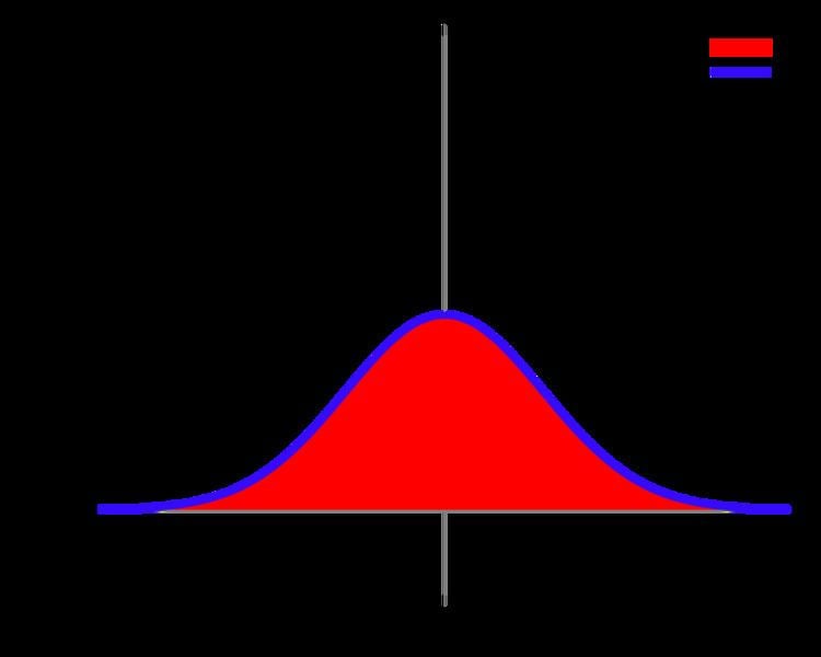
This integral has a wide range of applications. For example, with a slight change of variables it is used to compute the normalizing constant of the normal distribution. The same integral with finite limits is closely related both to the error function and the cumulative distribution function of the normal distribution. In physics this type of integral appears frequently, for example, in quantum mechanics, to find the probability density of the ground state of the harmonic oscillator, also in the path integral formulation, and to find the propagator of the harmonic oscillator, we make use of this integral.

Although no elementary function exists for the error function, as can be proven by the Risch algorithm, the Gaussian integral can be solved analytically through the methods of multivariable calculus. That is, there is no elementary indefinite integral for

∫ e − x 2 d x ,

but the definite integral

∫ − ∞ + ∞ e − x 2 d x

can be evaluated.

The Gaussian integral is encountered very often in physics and numerous generalizations of the integral are encountered in quantum field theory.

By polar coordinates

A standard way to compute the Gaussian integral, the idea of which goes back to Poisson, is to make use of the property that:

( ∫ − ∞ ∞ e − x 2 d x ) 2 = ∫ − ∞ ∞ e − x 2 d x ∫ − ∞ ∞ e − y 2 d y = ∫ − ∞ ∞ ∫ − ∞ ∞ e − ( x 2 + y 2 ) d x d y

consider the function e^{−(x² + y²)} = e^−r² on the plane R², and compute its integral two ways:

on the one hand, by double integration in the Cartesian coordinate system, its integral is a square:
on the other hand, by shell integration (a case of double integration in polar coordinates), its integral is computed to be π.

Comparing these two computations yields the integral, though one should take care about the improper integrals involved.

∬ R 2 e − ( x 2 + y 2 ) d ( x , y ) = ∫ 0 2 π ∫ 0 ∞ e − r 2 r d r d θ = 2 π ∫ 0 ∞ r e − r 2 d r = 2 π ∫ − ∞ 0 1 2 e s d s s = − r 2 = π ∫ − ∞ 0 e s d s = π ( e 0 − e − ∞ ) = π ,

where the factor of r comes from the transform to polar coordinates (r dr dθ is the standard measure on the plane, expressed in polar coordinates Wikibooks:Calculus/Polar Integration#Generalization), and the substitution involves taking s = −r², so ds = −2r dr.

Combining these yields

( ∫ − ∞ ∞ e − x 2 d x ) 2 = π ,

so

∫ − ∞ ∞ e − x 2 d x = π .

Careful proof

To justify the improper double integrals and equating the two expressions, we begin with an approximating function:

I ( a ) = ∫ − a a e − x 2 d x .

If the integral

∫ − ∞ ∞ e − x 2 d x

were absolutely convergent we would have that its Cauchy principal value, that is, the limit

lim a → ∞ I ( a )

would coincide with

∫ − ∞ ∞ e − x 2 d x .

To see that this is the case, consider that

∫ − ∞ ∞ | e − x 2 | d x < ∫ − ∞ − 1 − x e − x 2 d x + ∫ − 1 1 e − x 2 d x + ∫ 1 ∞ x e − x 2 d x < ∞ .

so we can compute

∫ − ∞ ∞ e − x 2 d x

by just taking the limit

lim a → ∞ I ( a ) .

Taking the square of I ( a ) yields

I ( a ) 2 = ( ∫ − a a e − x 2 d x ) ( ∫ − a a e − y 2 d y ) = ∫ − a a ( ∫ − a a e − y 2 d y ) e − x 2 d x = ∫ − a a ∫ − a a e − ( x 2 + y 2 ) d y d x .

Using Fubini's theorem, the above double integral can be seen as an area integral

∬ [ − a , a ] × [ − a , a ] e − ( x 2 + y 2 ) d ( x , y ) ,

taken over a square with vertices {(−a, a), (a, a), (a, −a), (−a, −a)} on the xy-plane.

Since the exponential function is greater than 0 for all real numbers, it then follows that the integral taken over the square's incircle must be less than I ( a ) 2 , and similarly the integral taken over the square's circumcircle must be greater than I ( a ) 2 . The integrals over the two disks can easily be computed by switching from cartesian coordinates to polar coordinates:

x = r cos ⁡ θ y = r sin ⁡ θ J ( r , θ ) = [ ∂ x ∂ r ∂ x ∂ θ ∂ y ∂ r ∂ y ∂ θ ] = [ cos ⁡ θ − r sin ⁡ θ sin ⁡ θ r cos ⁡ θ ] d ( x , y ) = | J ( r , θ ) | d ( r , θ ) = r d ( r , θ ) . ∫ 0 2 π ∫ 0 a r e − r 2 d r d θ < I 2 ( a ) < ∫ 0 2 π ∫ 0 a 2 r e − r 2 d r d θ .

(See to polar coordinates from Cartesian coordinates for help with polar transformation.)

Integrating,

π ( 1 − e − a 2 ) < I 2 ( a ) < π ( 1 − e − 2 a 2 ) .

By the squeeze theorem, this gives the Gaussian integral

∫ − ∞ ∞ e − x 2 d x = π .

By Cartesian coordinates

A different technique, which goes back to Laplace (1812), is the following. Let

y = x s d y = x d s .

Since the limits on s as y → ±∞ depend on the sign of x, it simplifies the calculation to use the fact that e^−x² is an even function, and, therefore, the integral over all real numbers is just twice the integral from zero to infinity. That is,

∫ − ∞ ∞ e − x 2 d x = 2 ∫ 0 ∞ e − x 2 d x .

Thus, over the range of integration, x ≥ 0, and the variables y and s have the same limits. This yields:

I 2 = 4 ∫ 0 ∞ ∫ 0 ∞ e − ( x 2 + y 2 ) d y d x = 4 ∫ 0 ∞ ( ∫ 0 ∞ e − ( x 2 + y 2 ) d y ) d x = 4 ∫ 0 ∞ ( ∫ 0 ∞ e − x 2 ( 1 + s 2 ) x d s ) d x = 4 ∫ 0 ∞ ( ∫ 0 ∞ e − x 2 ( 1 + s 2 ) x d x ) d s = 4 ∫ 0 ∞ [ 1 − 2 ( 1 + s 2 ) e − x 2 ( 1 + s 2 ) ] x = 0 x = ∞ d s = 4 ( 1 2 ∫ 0 ∞ d s 1 + s 2 ) = 2 [ arctan ⁡ s ] 0 ∞ = π

Therefore, I = π , as expected.

Relation to the gamma function

The integrand is an even function,

∫ − ∞ ∞ e − x 2 d x = 2 ∫ 0 ∞ e − x 2 d x

Thus, after the change of variable x = t , this turns into the Euler integral

2 ∫ 0 ∞ e − x 2 d x = 2 ∫ 0 ∞ 1 2 e − t t − 1 2 d t = Γ ( 1 2 ) = π

where Γ is the gamma function. This shows why the factorial of a half-integer is a rational multiple of π . More generally,

∫ 0 ∞ e − a x b d x = Γ ( 1 b ) b a 1 b

The integral of a Gaussian function

The integral of an arbitrary Gaussian function is

∫ − ∞ ∞ e − a ( x + b ) 2 d x = π a .

An alternative form is

∫ − ∞ ∞ e − a x 2 + b x + c d x = π a e b 2 4 a + c ,

This form is very useful in calculating mathematical expectations of some continuous probability distributions concerning normal distribution.

See, for example, the expectation of the log-normal distribution.

n-dimensional and functional generalization

Suppose A is a symmetric positive-definite (hence invertible) n × n precision matrix, which is the matrix inverse of the covariance matrix. Then,

∫ − ∞ ∞ e ( − 1 2 ∑ i , j = 1 n A i j x i x j ) d n x = ∫ − ∞ ∞ e ( − 1 2 x T A x ) d n x = ( 2 π ) n det A = 1 det ( A / 2 π ) = det ( 2 π A − 1 )

where the integral is understood to be over Rⁿ. This fact is applied in the study of the multivariate normal distribution.

Also,

∫ x k 1 ⋯ x k 2 N e ( − 1 2 ∑ i , j = 1 n A i j x i x j ) d n x = ( 2 π ) n det A 1 2 N N ! ∑ σ ∈ S 2 N ( A − 1 ) k σ ( 1 ) k σ ( 2 ) ⋯ ( A − 1 ) k σ ( 2 N − 1 ) k σ ( 2 N )

where σ is a permutation of {1, ..., 2N} and the extra factor on the right-hand side is the sum over all combinatorial pairings of {1, ..., 2N} of N copies of A⁻¹.

Alternatively,

∫ f ( x → ) e ( − 1 2 ∑ i , j = 1 n A i j x i x j ) d n x = ( 2 π ) n det A e ( 1 2 ∑ i , j = 1 n ( A − 1 ) i j ∂ ∂ x i ∂ ∂ x j ) f ( x → ) | x → = 0

for some analytic function f, provided it satisfies some appropriate bounds on its growth and some other technical criteria. (It works for some functions and fails for others. Polynomials are fine.) The exponential over a differential operator is understood as a power series.

While functional integrals have no rigorous definition (or even a nonrigorous computational one in most cases), we can define a Gaussian functional integral in analogy to the finite-dimensional case. There is still the problem, though, that ( 2 π ) ∞ is infinite and also, the functional determinant would also be infinite in general. This can be taken care of if we only consider ratios:

∫ f ( x 1 ) ⋯ f ( x 2 N ) e − ∬ 1 2 A ( x 2 N + 1 , x 2 N + 2 ) f ( x 2 N + 1 ) f ( x 2 N + 2 ) d d x 2 N + 1 d d x 2 N + 2 D f ∫ e − ∬ 1 2 A ( x 2 N + 1 , x 2 N + 2 ) f ( x 2 N + 1 ) f ( x 2 N + 2 ) d d x 2 N + 1 d d x 2 N + 2 D f = 1 2 N N ! ∑ σ ∈ S 2 N A − 1 ( x σ ( 1 ) , x σ ( 2 ) ) ⋯ A − 1 ( x σ ( 2 N − 1 ) , x σ ( 2 N ) ) .

In the DeWitt notation, the equation looks identical to the finite-dimensional case.

n-dimensional with linear term

If A is again a symmetric positive-definite matrix, then (assuming all are column vectors)

∫ e − 1 2 ∑ i , j = 1 n A i j x i x j + ∑ i = 1 n B i x i d n x = ∫ e − 1 2 x → T A x → + B → T x → d n x = ( 2 π ) n det A e 1 2 B → T A − 1 B → .

Integrals of similar form

∫ 0 ∞ x 2 n e − x 2 a 2 d x = π a 2 n + 1 ( 2 n − 1 ) ! ! 2 n + 1 ∫ 0 ∞ x 2 n + 1 e − x 2 a 2 d x = n ! 2 a 2 n + 2 ∫ 0 ∞ x 2 n e − a x 2 d x = ( 2 n − 1 ) ! ! a n 2 n + 1 π a ∫ 0 ∞ x 2 n + 1 e − a x 2 d x = n ! 2 a n + 1 ∫ 0 ∞ x n e − a x 2 d x = Γ ( ( n + 1 ) 2 ) 2 a ( n + 1 ) 2

(n positive integer)

An easy way to derive these is by parameter differentiation.

∫ − ∞ ∞ x 2 n e − α x 2 d x = ( − 1 ) n ∫ − ∞ ∞ ∂ n ∂ α n e − α x 2 d x = ( − 1 ) n ∂ n ∂ α n ∫ − ∞ ∞ e − α x 2 d x = π ( − 1 ) n ∂ n ∂ α n α − 1 2 = π α ( 2 n − 1 ) ! ! ( 2 α ) n

One could also integrate by parts and find a recurrence relation to solve this.

Higher-order polynomials

Applying a linear change of basis shows that the integral of the exponential of a homogeneous polynomial in n variables may depend only on SL(n)-invariants of the polynomial. One such invariant is the discriminant, zeros of which mark the singularities of the integral. However, the integral may also depend on other invariants.

Exponentials of other even polynomials can numerically be solved using series. For example the solution to the integral of the exponential of a quartic polynomial is

∫ − ∞ ∞ e a x 4 + b x 3 + c x 2 + d x + f d x = 1 2 e f ∑ n , m , p = 0 n + p = 0 mod 2 ∞ b n n ! c m m ! d p p ! Γ ( 3 n + 2 m + p + 1 4 ) ( − a ) 3 n + 2 m + p + 1 4 .

The n + p = 0 mod 2 requirement is because the integral from −∞ to 0 contributes a factor of (−1)^n+p/2 to each term, while the integral from 0 to +∞ contributes a factor of 1/2 to each term. These integrals turn up in subjects such as quantum field theory.

References

Gaussian integral Wikipedia

(Text) CC BY-SA

Contents