Antiderivative

Example

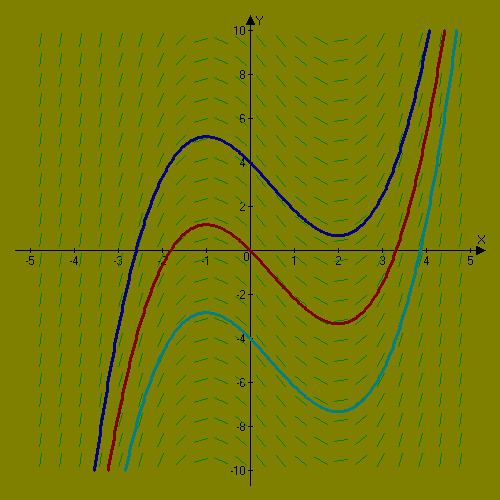
The function F(x) = x³/3 is an antiderivative of f(x) = x², as the derivative of x³/3 is x². As the derivative of a constant is zero, x² will have an infinite number of antiderivatives, such as x³/3, x³/3 + 1, x³/3 - 2, etc. Thus, all the antiderivatives of x² can be obtained by changing the value of C in F(x) = x³/3 + C; where C is an arbitrary constant known as the constant of integration. Essentially, the graphs of antiderivatives of a given function are vertical translations of each other; each graph's vertical location depending upon the value of C.

In physics, the integration of acceleration yields velocity plus a constant. The constant is the initial velocity term that would be lost upon taking the derivative of velocity because the derivative of a constant term is zero. This same pattern applies to further integrations and derivatives of motion (position, velocity, acceleration, and so on).

Uses and properties

Antiderivatives are important because they can be used to compute definite integrals, using the fundamental theorem of calculus: if F is an antiderivative of the integrable function f over the interval [a, b], then:

∫ a b f ( x ) d x = F ( b ) − F ( a ) .

Because of this, each of the infinitely many antiderivatives of a given function f is sometimes called the "general integral" or "indefinite integral" of f and is written using the integral symbol with no bounds:

∫ f ( x ) d x .

If F is an antiderivative of f, and the function f is defined on some interval, then every other antiderivative G of f differs from F by a constant: there exists a number C such that G(x) = F(x) + C for all x. C is called the arbitrary constant of integration. If the domain of F is a disjoint union of two or more intervals, then a different constant of integration may be chosen for each of the intervals. For instance

F ( x ) = { − 1 x + C 1 x < 0 − 1 x + C 2 x > 0

is the most general antiderivative of f ( x ) = 1 / x 2 on its natural domain ( − ∞ , 0 ) ∪ ( 0 , ∞ ) .

Every continuous function f has an antiderivative, and one antiderivative F is given by the definite integral of f with variable upper boundary:

F ( x ) = ∫ 0 x f ( t ) d t .

Varying the lower boundary produces other antiderivatives (but not necessarily all possible antiderivatives). This is another formulation of the fundamental theorem of calculus.

There are many functions whose antiderivatives, even though they exist, cannot be expressed in terms of elementary functions (like polynomials, exponential functions, logarithms, trigonometric functions, inverse trigonometric functions and their combinations). Examples of these are

∫ e − x 2 d x , ∫ sin ⁡ x 2 d x , ∫ sin ⁡ x x d x , ∫ 1 ln ⁡ x d x , ∫ x x d x .

From left to right, the first four are the error function, the Fresnel function, the trigonometric integral, and the logarithmic integral function.

See also Differential Galois theory for a more detailed discussion.

Techniques of integration

Finding antiderivatives of elementary functions is often considerably harder than finding their derivatives. For some elementary functions, it is impossible to find an antiderivative in terms of other elementary functions. See the articles on elementary functions and nonelementary integral for further information.

There are various methods available:

the linearity of integration allows us to break complicated integrals into simpler ones

integration by substitution, often combined with trigonometric identities or the natural logarithm

the inverse chain rule method, a special case of integration by substitution

integration by parts to integrate products of functions

Inverse function integration, a formula that expresses the antiderivative of the inverse f − 1 of an invertible and continuous function f in terms of the antiderivative of f and of f − 1 .

the method of partial fractions in integration allows us to integrate all rational functions (fractions of two polynomials)

the Risch algorithm

when integrating multiple times, certain additional techniques can be used, see for instance double integrals and polar coordinates, the Jacobian and the Stokes' theorem

if a function has no elementary antiderivative (for instance, exp(-x²)), its definite integral can be approximated using numerical integration

it is often convenient to algebraically manipulate the integrand such that other integration techniques, such as integration by substitution, may be used.

to calculate the (n times) repeated antiderivative of a function f, Cauchy's formula is useful (cf. Cauchy formula for repeated integration):

Computer algebra systems can be used to automate some or all of the work involved in the symbolic techniques above, which is particularly useful when the algebraic manipulations involved are very complex or lengthy. Integrals which have already been derived can be looked up in a table of integrals.

Antiderivatives of non-continuous functions

Non-continuous functions can have antiderivatives. While there are still open questions in this area, it is known that:

Some highly pathological functions with large sets of discontinuities may nevertheless have antiderivatives.

In some cases, the antiderivatives of such pathological functions may be found by Riemann integration, while in other cases these functions are not Riemann integrable.

Assuming that the domains of the functions are open intervals:

A necessary, but not sufficient, condition for a function f to have an antiderivative is that f have the intermediate value property. That is, if [a, b] is a subinterval of the domain of f and C is any real number between f(a) and f(b), then f(c) = C for some c between a and b. This is a consequence of Darboux's theorem.

The set of discontinuities of f must be a meagre set. This set must also be an F-sigma set (since the set of discontinuities of any function must be of this type). Moreover, for any meagre F-sigma set, one can construct some function f having an antiderivative, which has the given set as its set of discontinuities.

If f has an antiderivative, is bounded on closed finite subintervals of the domain and has a set of discontinuities of Lebesgue measure 0, then an antiderivative may be found by integration in the sense of Lebesgue. In fact, using more powerful integrals like the Henstock–Kurzweil integral, every function for which an antiderivative exists is integrable, and its general integral coincides with its antiderivative.

If f has an antiderivative F on a closed interval [a,b], then for any choice of partition a = x 0 < x 1 < x 2 < ⋯ < x n = b , if one chooses sample points x i ∗ ∈ [ x i − 1 , x i ] as specified by the mean value theorem, then the corresponding Riemann sum telescopes to the value F(b) − F(a).

∑ i = 1 n f ( x i ∗ ) ( x i − x i − 1 ) = ∑ i = 1 n [ F ( x i ) − F ( x i − 1 ) ] = F ( x n ) − F ( x 0 ) = F ( b ) − F ( a ) However if f is unbounded, or if f is bounded but the set of discontinuities of f has positive Lebesgue measure, a different choice of sample points x i ∗ may give a significantly different value for the Riemann sum, no matter how fine the partition. See Example 4 below.