
 | ||
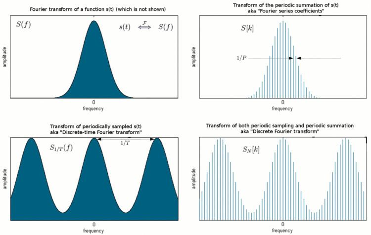
In mathematics, the discrete Fourier transform (DFT) converts a finite sequence of equally-spaced samples of a function into an equivalent-length sequence of equally-spaced samples of the discrete-time Fourier transform (DTFT), which is a complex-valued function of frequency . The interval at which the DTFT is sampled is the reciprocal of the duration of the input sequence. An inverse DFT is a Fourier series, using the DTFT samples as coefficients of complex sinusoids at the corresponding DTFT frequencies. It has the same sample-values as the original input sequence. The DFT is therefore said to be a frequency domain representation of the original input sequence. If the original sequence spans all the non-zero values of a function, its DTFT is continuous (and periodic), and the DFT provides discrete samples of one cycle. If the original sequence is one cycle of a periodic function, the DFT provides all the non-zero values of one DTFT cycle.
Contents
- Definition
- Completeness
- Orthogonality
- The Plancherel theorem and Parsevals theorem
- Periodicity
- Shift theorem
- Convolution theorem duality
- Trigonometric interpolation polynomial
- The unitary DFT
- Expressing the inverse DFT in terms of the DFT
- Eigenvalues and eigenvectors
- Uncertainty principle
- The real input DFT
- Generalized DFT shifted and non linear phase
- Multidimensional DFT
- The real input multidimensional DFT
- Applications
- Spectral analysis
- Filter bank
- Data compression
- Partial differential equations
- Polynomial multiplication
- Multiplication of large integers
- Convolution
- Representation theory
- Other fields
- Other finite groups
- Alternatives
- References
The DFT is the most important discrete transform, used to perform Fourier analysis in many practical applications. In digital signal processing, the function is any quantity or signal that varies over time, such as the pressure of a sound wave, a radio signal, or daily temperature readings, sampled over a finite time interval (often defined by a window function). In image processing, the samples can be the values of pixels along a row or column of a raster image. The DFT is also used to efficiently solve partial differential equations, and to perform other operations such as convolutions or multiplying large integers.
Since it deals with a finite amount of data, it can be implemented in computers by numerical algorithms or even dedicated hardware. These implementations usually employ efficient fast Fourier transform (FFT) algorithms; so much so that the terms "FFT" and "DFT" are often used interchangeably. Prior to its current usage, the "FFT" initialism may have also been used for the ambiguous term "finite Fourier transform".
Definition
The sequence of N complex numbers
Because of periodicity, the customary domain of k actually computed is [0, N − 1]. That is always the case when the DFT is implemented via the Fast Fourier transform algorithm. But other common domains are [−N/2, N/2 − 1] (N even) and [−(N − 1)/2, (N − 1)/2] (N odd), as when the left and right halves of an FFT output sequence are swapped.
The transform is sometimes denoted by the symbol
Eq.1 can be interpreted or derived in various ways, for example:
The normalization factor multiplying the DFT and IDFT (here 1 and 1/N) and the signs of the exponents are merely conventions, and differ in some treatments. The only requirements of these conventions are that the DFT and IDFT have opposite-sign exponents and that the product of their normalization factors be 1/N. A normalization of
In the following discussion the terms "sequence" and "vector" will be considered interchangeable.
Using Euler's formula, the DFT formulae can be converted to the trigonometric forms sometimes used in engineering and computer science:
Fourier Transform:
Inverse Fourier Transform:
Completeness
The discrete Fourier transform is an invertible, linear transformation
with
Orthogonality
The vectors
where
The Plancherel theorem and Parseval's theorem
If Xk and Yk are the DFTs of xn and yn respectively then the Parseval's theorem states:
where the star denotes complex conjugation. Plancherel theorem is a special case of the Parseval's theorem and states:
These theorems are also equivalent to the unitary condition below.
Periodicity
The periodicity can be shown directly from the definition:
Similarly, it can be shown that the IDFT formula leads to a periodic extension.
Shift theorem
Multiplying
The convolution theorem for the discrete-time Fourier transform indicates that a convolution of two infinite sequences can be obtained as the inverse transform of the product of the individual transforms. An important simplification occurs when the sequences are of finite length, N. In terms of the DFT and inverse DFT, it can be written as follows:
which is the convolution of the
Similarly, the cross-correlation of
When either sequence contains a string of zeros, of length L, L+1 of the circular convolution outputs are equivalent to values of
Convolution theorem duality
It can also be shown that:
Trigonometric interpolation polynomial
The trigonometric interpolation polynomial
where the coefficients Xk are given by the DFT of xn above, satisfies the interpolation property
For even N, notice that the Nyquist component
This interpolation is not unique: aliasing implies that one could add N to any of the complex-sinusoid frequencies (e.g. changing
In contrast, the most obvious trigonometric interpolation polynomial is the one in which the frequencies range from 0 to
The unitary DFT
Another way of looking at the DFT is to note that in the above discussion, the DFT can be expressed as the DFT matrix, a Vandermonde matrix, introduced by Sylvester in 1867,
where
is a primitive Nth root of unity.
The inverse transform is then given by the inverse of the above matrix,
With unitary normalization constants
where det() is the determinant function. The determinant is the product of the eigenvalues, which are always
The orthogonality of the DFT is now expressed as an orthonormality condition (which arises in many areas of mathematics as described in root of unity):
If X is defined as the unitary DFT of the vector x, then
and the Plancherel theorem is expressed as
If we view the DFT as just a coordinate transformation which simply specifies the components of a vector in a new coordinate system, then the above is just the statement that the dot product of two vectors is preserved under a unitary DFT transformation. For the special case
A consequence of the circular convolution theorem is that the DFT matrix F diagonalizes any circulant matrix.
Expressing the inverse DFT in terms of the DFT
A useful property of the DFT is that the inverse DFT can be easily expressed in terms of the (forward) DFT, via several well-known "tricks". (For example, in computations, it is often convenient to only implement a fast Fourier transform corresponding to one transform direction and then to get the other transform direction from the first.)
First, we can compute the inverse DFT by reversing all but one of the inputs (Duhamel et al., 1988):
(As usual, the subscripts are interpreted modulo N; thus, for
Second, one can also conjugate the inputs and outputs:
Third, a variant of this conjugation trick, which is sometimes preferable because it requires no modification of the data values, involves swapping real and imaginary parts (which can be done on a computer simply by modifying pointers). Define swap(
That is, the inverse transform is the same as the forward transform with the real and imaginary parts swapped for both input and output, up to a normalization (Duhamel et al., 1988).
The conjugation trick can also be used to define a new transform, closely related to the DFT, that is involutory—that is, which is its own inverse. In particular,
Eigenvalues and eigenvectors
The eigenvalues of the DFT matrix are simple and well-known, whereas the eigenvectors are complicated, not unique, and are the subject of ongoing research.
Consider the unitary form
This matrix satisfies the matrix polynomial equation:
This can be seen from the inverse properties above: operating
Therefore, the eigenvalues of
Since there are only four distinct eigenvalues for this
The problem of their multiplicity was solved by McClellan and Parks (1972), although it was later shown to have been equivalent to a problem solved by Gauss (Dickinson and Steiglitz, 1982). The multiplicity depends on the value of N modulo 4, and is given by the following table:
Otherwise stated, the characteristic polynomial of
No simple analytical formula for general eigenvectors is known. Moreover, the eigenvectors are not unique because any linear combination of eigenvectors for the same eigenvalue is also an eigenvector for that eigenvalue. Various researchers have proposed different choices of eigenvectors, selected to satisfy useful properties like orthogonality and to have "simple" forms (e.g., McClellan and Parks, 1972; Dickinson and Steiglitz, 1982; Grünbaum, 1982; Atakishiyev and Wolf, 1997; Candan et al., 2000; Hanna et al., 2004; Gurevich and Hadani, 2008).
A straightforward approach is to discretize an eigenfunction of the continuous Fourier transform, of which the most famous is the Gaussian function. Since periodic summation of the function means discretizing its frequency spectrum and discretization means periodic summation of the spectrum, the discretized and periodically summed Gaussian function yields an eigenvector of the discrete transform:
Two other simple closed-form analytical eigenvectors for special DFT period N were found (Kong, 2008):
For DFT period N = 2L + 1 = 4K +1, where K is an integer, the following is an eigenvector of DFT:
For DFT period N = 2L = 4K, where K is an integer, the following is an eigenvector of DFT:
The choice of eigenvectors of the DFT matrix has become important in recent years in order to define a discrete analogue of the fractional Fourier transform—the DFT matrix can be taken to fractional powers by exponentiating the eigenvalues (e.g., Rubio and Santhanam, 2005). For the continuous Fourier transform, the natural orthogonal eigenfunctions are the Hermite functions, so various discrete analogues of these have been employed as the eigenvectors of the DFT, such as the Kravchuk polynomials (Atakishiyev and Wolf, 1997). The "best" choice of eigenvectors to define a fractional discrete Fourier transform remains an open question, however.
Uncertainty principle
If the random variable Xk is constrained by
then
may be considered to represent a discrete probability mass function of n, with an associated probability mass function constructed from the transformed variable,
For the case of continuous functions
where
However, the Hirschman entropic uncertainty will have a useful analog for the case of the DFT. The Hirschman uncertainty principle is expressed in terms of the Shannon entropy of the two probability functions.
In the discrete case, the Shannon entropies are defined as
and
and the entropic uncertainty principle becomes
The equality is obtained for
There is also a well-known deterministic uncertainty principle that uses signal sparsity (or the number of non-zero coefficients). Let
As an immediate consequence of the inequality of arithmetic and geometric means, one also has
The real-input DFT
If
It follows that X0 and XN/2 are real-valued, and the remainder of the DFT is completely specified by just N/2-1 complex numbers.
Generalized DFT (shifted and non-linear phase)
It is possible to shift the transform sampling in time and/or frequency domain by some real shifts a and b, respectively. This is sometimes known as a generalized DFT (or GDFT), also called the shifted DFT or offset DFT, and has analogous properties to the ordinary DFT:
Most often, shifts of
Another interesting choice is
The term GDFT is also used for the non-linear phase extensions of DFT. Hence, GDFT method provides a generalization for constant amplitude orthogonal block transforms including linear and non-linear phase types. GDFT is a framework to improve time and frequency domain properties of the traditional DFT, e.g. auto/cross-correlations, by the addition of the properly designed phase shaping function (non-linear, in general) to the original linear phase functions (Akansu and Agirman-Tosun, 2010).
The discrete Fourier transform can be viewed as a special case of the z-transform, evaluated on the unit circle in the complex plane; more general z-transforms correspond to complex shifts a and b above.
Multidimensional DFT
The ordinary DFT transforms a one-dimensional sequence or array
where
where the division
The inverse of the multi-dimensional DFT is, analogous to the one-dimensional case, given by:
As the one-dimensional DFT expresses the input
The multidimensional DFT can be computed by the composition of a sequence of one-dimensional DFTs along each dimension. In the two-dimensional case
An algorithm to compute a one-dimensional DFT is thus sufficient to efficiently compute a multidimensional DFT. This approach is known as the row-column algorithm. There are also intrinsically multidimensional FFT algorithms.
The real-input multidimensional DFT
For input data
where the star again denotes complex conjugation and the
Applications
The DFT has seen wide usage across a large number of fields; we only sketch a few examples below (see also the references at the end). All applications of the DFT depend crucially on the availability of a fast algorithm to compute discrete Fourier transforms and their inverses, a fast Fourier transform.
Spectral analysis
When the DFT is used for signal spectral analysis, the
A final source of distortion (or perhaps illusion) is the DFT itself, because it is just a discrete sampling of the DTFT, which is a function of a continuous frequency domain. That can be mitigated by increasing the resolution of the DFT. That procedure is illustrated at Sampling the DTFT.
Filter bank
See FFT filter banks and Sampling the DTFT.
Data compression
The field of digital signal processing relies heavily on operations in the frequency domain (i.e. on the Fourier transform). For example, several lossy image and sound compression methods employ the discrete Fourier transform: the signal is cut into short segments, each is transformed, and then the Fourier coefficients of high frequencies, which are assumed to be unnoticeable, are discarded. The decompressor computes the inverse transform based on this reduced number of Fourier coefficients. (Compression applications often use a specialized form of the DFT, the discrete cosine transform or sometimes the modified discrete cosine transform.) Some relatively recent compression algorithms, however, use wavelet transforms, which give a more uniform compromise between time and frequency domain than obtained by chopping data into segments and transforming each segment. In the case of JPEG2000, this avoids the spurious image features that appear when images are highly compressed with the original JPEG.
Partial differential equations
Discrete Fourier transforms are often used to solve partial differential equations, where again the DFT is used as an approximation for the Fourier series (which is recovered in the limit of infinite N). The advantage of this approach is that it expands the signal in complex exponentials
Polynomial multiplication
Suppose we wish to compute the polynomial product c(x) = a(x) · b(x). The ordinary product expression for the coefficients of c involves a linear (acyclic) convolution, where indices do not "wrap around." This can be rewritten as a cyclic convolution by taking the coefficient vectors for a(x) and b(x) with constant term first, then appending zeros so that the resultant coefficient vectors a and b have dimension d > deg(a(x)) + deg(b(x)). Then,
Where c is the vector of coefficients for c(x), and the convolution operator
But convolution becomes multiplication under the DFT:
Here the vector product is taken elementwise. Thus the coefficients of the product polynomial c(x) are just the terms 0, ..., deg(a(x)) + deg(b(x)) of the coefficient vector
With a fast Fourier transform, the resulting algorithm takes O (N log N) arithmetic operations. Due to its simplicity and speed, the Cooley–Tukey FFT algorithm, which is limited to composite sizes, is often chosen for the transform operation. In this case, d should be chosen as the smallest integer greater than the sum of the input polynomial degrees that is factorizable into small prime factors (e.g. 2, 3, and 5, depending upon the FFT implementation).
Multiplication of large integers
The fastest known algorithms for the multiplication of very large integers use the polynomial multiplication method outlined above. Integers can be treated as the value of a polynomial evaluated specifically at the number base, with the coefficients of the polynomial corresponding to the digits in that base. After polynomial multiplication, a relatively low-complexity carry-propagation step completes the multiplication.
Convolution
When data is convolved with a function with wide support, such as for downsampling by a large sampling ratio, because of the Convolution theorem and the FFT algorithm, it may be faster to transform it, multiply pointwise by the transform of the filter and then reverse transform it. Alternatively, a good filter is obtained by simply truncating the transformed data and re-transforming the shortened data set.
Representation theory
The DFT can be interpreted as the complex-valued representation theory of the finite cyclic group. In other words, a sequence of n complex numbers can be thought of as an element of n-dimensional complex space Cn or equivalently a function f from the finite cyclic group of order n to the complex numbers, Zn → C. So f is a class function on the finite cyclic group, and thus can be expressed as a linear combination of the irreducible characters of this group, which are the roots of unity.
From this point of view, one may generalize the DFT to representation theory generally, or more narrowly to the representation theory of finite groups.
More narrowly still, one may generalize the DFT by either changing the target (taking values in a field other than the complex numbers), or the domain (a group other than a finite cyclic group), as detailed in the sequel.
Other fields
Many of the properties of the DFT only depend on the fact that
Other finite groups
The standard DFT acts on a sequence x0, x1, …, xN−1 of complex numbers, which can be viewed as a function {0, 1, …, N − 1} → C. The multidimensional DFT acts on multidimensional sequences, which can be viewed as functions
This suggests the generalization to Fourier transforms on arbitrary finite groups, which act on functions G → C where G is a finite group. In this framework, the standard DFT is seen as the Fourier transform on a cyclic group, while the multidimensional DFT is a Fourier transform on a direct sum of cyclic groups.
Alternatives
There are various alternatives to the DFT for various applications, prominent among which are wavelets. The analog of the DFT is the discrete wavelet transform (DWT). From the point of view of time–frequency analysis, a key limitation of the Fourier transform is that it does not include location information, only frequency information, and thus has difficulty in representing transients. As wavelets have location as well as frequency, they are better able to represent location, at the expense of greater difficulty representing frequency. For details, see comparison of the discrete wavelet transform with the discrete Fourier transform.