Discrete time Fourier transform - Alchetron, the free social encyclopedia

In mathematics, the discrete-time Fourier transform (DTFT) is a form of Fourier analysis that is applicable to the uniformly-spaced samples of a continuous function. The term discrete-time refers to the fact that the transform operates on discrete data (samples) whose interval often has units of time. From only the samples, it produces a function of frequency that is a periodic summation of the continuous Fourier transform of the original continuous function. Under certain theoretical conditions, described by the sampling theorem, the original continuous function can be recovered perfectly from the DTFT and thus from the original discrete samples. The DTFT itself is a continuous function of frequency, but discrete samples of it can be readily calculated via the discrete Fourier transform (DFT) (see Sampling the DTFT), which is by far the most common method of modern Fourier analysis.

Definition

The discrete-time Fourier transform of a discrete set of real or complex numbers x[n], for all integers n, is a Fourier series, which produces a periodic function of a frequency variable. When the frequency variable, ω, has normalized units of radians/sample, the periodicity is 2π, and the Fourier series is:

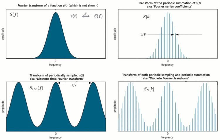
The utility of this frequency domain function is rooted in the Poisson summation formula. Let X(f) be the Fourier transform of any function, x(t), whose samples at some interval T (seconds) are equal (or proportional to) the x[n] sequence, i.e. T ⋅ x ( n T ) = x [ n ] . Then the periodic function represented by the Fourier series is a periodic summation of X(f). In terms of frequency f in hertz (cycles/sec):

The integer k has units of cycles/sample, and 1/T is the sample-rate, f_s (samples/sec). So X_1/T(f) comprises exact copies of X(f) that are shifted by multiples of f_s hertz and combined by addition. For sufficiently large f_s the k=0 term can be observed in the region [−f_s/2, f_s/2] with little or no distortion (aliasing) from the other terms. In Fig.1, the extremities of the distribution in the upper left corner are masked by aliasing in the periodic summation (lower left).

We also note that e − i 2 π f T n is the Fourier transform of δ ( t − n T ) . Therefore, an alternative definition of DTFT is:

The modulated Dirac comb function is a mathematical abstraction sometimes referred to as impulse sampling.

Inverse transform

An operation that recovers the discrete data sequence from the DTFT function is called an inverse DTFT. For instance, the inverse continuous Fourier transform of both sides of Eq.3 produces the sequence in the form of a modulated Dirac comb function:

∑ n = − ∞ ∞ x [ n ] ⋅ δ ( t − n T ) = F − 1 { X 1 / T ( f ) } = d e f ∫ − ∞ ∞ X 1 / T ( f ) ⋅ e i 2 π f t d f .

However, noting that X_1/T(f) is periodic, all the necessary information is contained within any interval of length 1/T. In both Eq.1 and Eq.2, the summations over n are a Fourier series, with coefficients x[n]. The standard formulas for the Fourier coefficients are also the inverse transforms:

x [ n ] = T ∫ 1 T X 1 / T ( f ) ⋅ e i 2 π f n T d f (integral over any interval of length 1 / T ) = 1 2 π ∫ 2 π X 2 π ( ω ) ⋅ e i ω n d ω (integral over any interval of length 2 π )

Periodic data

When the input data sequence x[n] is N-periodic, Eq.2 can be computationally reduced to a discrete Fourier transform (DFT), because:

All the available information is contained within N samples.

X 1 / T ( f ) converges to zero everywhere except integer multiples of 1 N T , known as harmonic frequencies.

The DTFT is periodic, so the maximum number of unique harmonic amplitudes is 1 T / 1 N T = N .

The kernel x [ n ] ⋅ e − i 2 π f T n is N-periodic at the harmonic frequencies, f = k N T . Introducing the notation ∑ N to represent a sum over any n-sequence of length N, we can write:

X 1 / T ( k N T ) = ∑ m = − ∞ ∞ ( ∑ N x [ n − m N ] ⋅ e − i 2 π k N ( n − m N ) ) = ∑ m = − ∞ ∞ ( ∑ N x [ n ] ⋅ e − i 2 π k N n ) = T ( ∑ N x ( n T ) ⋅ e − i 2 π k N n ) ⏟ X [ k ] (DFT) ⋅ ( ∑ m = − ∞ ∞ 1 ) .

Therefore, the DTFT diverges at the harmonic frequencies, but at different frequency-dependent rates. And those rates are given by the DFT of one cycle of the x[n] sequence. In terms of a Dirac comb function, this is represented by:

X 1 / T ( f ) = ∑ k = − ∞ ∞ ( T ⋅ X [ k ] ) ⋅ 1 N T δ ( f − k N T ) = 1 N ∑ k = − ∞ ∞ X [ k ] ⋅ δ ( f − k N T ) ⏟ DTFT of a periodic sequence .

Sampling the DTFT

When the DTFT is continuous, a common practice is to compute an arbitrary number of samples (N) of one cycle of the periodic function X_1/T:

X 1 / T ( k N T ) ⏟ X k = ∑ n = − ∞ ∞ x [ n ] ⋅ e − i 2 π k n N k = 0 , … , N − 1 = ∑ N x N [ n ] ⋅ e − i 2 π k n N , ⏟ D F T (sum over any n -sequence of length N )

where x_N is a periodic summation:

x N [ n ] = def ∑ m = − ∞ ∞ x [ n − m N ] .

The x_N sequence is the inverse DFT. Thus, our sampling of the DTFT causes the inverse transform to become periodic. The array of | X k | 2 is known as a periodogram, where parameter N is known to Matlab users as NFFT.

In order to evaluate one cycle of x_N numerically, we require a finite-length x[n] sequence. For instance, a long sequence might be truncated by a window function of length L resulting in two cases worthy of special mention: L ≤ N and L = I•N, for some integer I (typically 6 or 8). For notational simplicity, consider the x[n] values below to represent the modified values.

When L = I•N a cycle of x_N reduces to a summation of I blocks of length N. This goes by various names, such as:

window-presum FFT

Weight, OverLap, Add (WOLA)

polyphase FFT

multiple block windowing

time-aliasing.

An interesting way to understand/motivate the technique is to recall that decimation of sampled data in one domain (time or frequency) produces aliasing in the other, and vice versa. The x_N summation is mathematically equivalent to aliasing, leading to decimation in frequency, leaving only DTFT samples least affected by spectral leakage. That is usually a priority when implementing an FFT filter-bank (channelizer). With a conventional window function of length L, scalloping loss would be unacceptable. So multi-block windows are created using FIR filter design tools. Their frequency profile is flat at the highest point and falls off quickly at the midpoint between the remaining DTFT samples. The larger the value of parameter I the better the potential performance. We note that the same results can be obtained by computing and decimating an L-length DFT, but that is not computationally efficient.

When L ≤ N the DFT is usually written in this more familiar form:

X k = ∑ n = 0 N − 1 x [ n ] ⋅ e − i 2 π k n N .

In order to take advantage of a fast Fourier transform algorithm for computing the DFT, the summation is usually performed over all N terms, even though N-L of them are zeros. Therefore, the case L < N is often referred to as "zero-padding".

Spectral leakage, which increases as L decreases, is detrimental to certain important performance metrics, such as resolution of multiple frequency components and the amount of noise measured by each DTFT sample. But those things don't always matter, for instance when the x[n] sequence is a noiseless sinusoid (or a constant), shaped by a window function. Then it is a common practice to use zero-padding to graphically display and compare the detailed leakage patterns of window functions. To illustrate that for a rectangular window, consider the sequence:

x [ n ] = e i 2 π 1 8 n , and L = 64.

The two figures below are plots of the magnitude of two different sized DFTs, as indicated in their labels. In both cases, the dominant component is at the signal frequency: f = 1/8 = 0.125. Also visible on the right is the spectral leakage pattern of the L = 64 rectangular window. The illusion on the left is a result of sampling the DTFT at all of its zero-crossings. Rather than the DTFT of a finite-length sequence, it gives the impression of an infinitely long sinusoidal sequence. Contributing factors to the illusion are the use of a rectangular window, and the choice of a frequency (1/8 = 8/64) with exactly 8 (an integer) cycles per 64 samples.

Convolution

The convolution theorem for sequences is:

x ∗ y = DTFT − 1 [ DTFT { x } ⋅ DTFT { y } ] .

An important special case is the circular convolution of sequences x and y defined by x_N * y where x_N is a periodic summation. The discrete-frequency nature of DTFT{x_N} "selects" only discrete values from the continuous function DTFT{y}, which results in considerable simplification of the inverse transform. As shown at Convolution theorem#Functions of discrete variable sequences:

x N ∗ y = DTFT − 1 [ DTFT { x N } ⋅ DTFT { y } ] = DFT − 1 [ DFT { x N } ⋅ DFT { y N } ] .

For x and y sequences whose non-zero duration is less than or equal to N, a final simplification is:

x N ∗ y = DFT − 1 [ DFT { x } ⋅ DFT { y } ] .

The significance of this result is expounded at Circular convolution and Fast convolution algorithms.

Relationship to the Z-transform

The bilateral Z-transform is defined by:

Z { x [ n ] } ⏟ X ^ ( z ) = ∑ n = − ∞ ∞ x [ n ] z − n , where z is a complex variable.

We denote this function as X ^ ( z ) to avoid confusion with the Fourier transform. For the special case that z is constrained to values of the form e i ω :

X ^ ( e i ω ) = ∑ n = − ∞ ∞ x [ n ] e − i ω n = X 2 π ( ω ) = X 1 / T ( ω 2 π T ) = ∑ k = − ∞ ∞ X ( ω 2 π T − k / T ) = ∑ k = − ∞ ∞ X ( ω − 2 π k 2 π T )

Note that when parameter T changes, the terms of X 2 π ( ω ) remain a constant separation (2π) apart, and their width scales up or down. The terms of X 1 / T ( f ) remain a constant width and their separation (1/T) scales up or down.

Table of discrete-time Fourier transforms

Some common transform pairs are shown in the table below. The following notation applies:

ω = 2πfT is a real number representing continuous angular frequency (in radians per sample). (f is in cycles/sec, and T is in sec/sample.) In all cases in the table, the DTFT is 2π-periodic (in ω).

X_2π(ω) designates a function defined on −∞ < ω < ∞.

X_o(ω) designates a function defined on −π < ω ≤ π, and zero elsewhere. Then:

δ(ω) is the Dirac delta function

sinc(t) is the normalized sinc function

rect(t) is the rectangle function

tri(t) is the triangle function

n is an integer representing the discrete-time domain (in samples)

u[n] is the discrete-time unit step function

δ[n] is the Kronecker delta δ_{n, 0}

Properties

This table shows some mathematical operations in the time domain and the corresponding effects in the frequency domain.

∗ is the discrete convolution of two sequences

x[n]* is the complex conjugate of x[n]

References

Discrete-time Fourier transform Wikipedia

(Text) CC BY-SA

Contents