Fractional Fourier transform

Introduction

The continuous Fourier transform F of a function ƒ: R → C is a unitary operator of L² that maps the function ƒ to its frequential version ƒ̂:

f ^ ( ξ ) = ∫ − ∞ ∞ f ( x )   e − 2 π i x ξ d x ,   for every real number ξ ,

and ƒ is determined by ƒ̂ via the inverse transform F − 1

f ( x ) = ∫ − ∞ ∞ f ^ ( ξ )   e 2 π i ξ x d ξ ,   for every real number x.

Let us study its n-th iterated F n defined by F n [ f ] = F [ F n − 1 [ f ] ] and F − n = ( F − 1 ) n when n is a non-negative integer, and F 0 [ f ] = f . Their sequence is finite since F is a 4-periodic automorphism: for every function ƒ, F 4 [ f ] = f .

More precisely, let us introduce the parity operator P that inverts time, P [ f ] : t ↦ f ( − t ) . Then the following properties hold:

F 0 = I d , F 1 = F , F 2 = P , F 4 = I d F 3 = F − 1 = P ∘ F = F ∘ P .

The FrFT provides a family of linear transforms that further extends this definition to handle non-integer powers n = 2α/π of the FT.

Definition

For any real α, the α-angle fractional Fourier transform of a function ƒ is denoted by F α ( u ) and defined by

(the square root is defined such that the argument of result lies in the interval [ − π / 2 , π / 2 ] ).

If α is an integer multiple of π, then the cotangent and cosecant functions above diverge. However, this can be handled by taking the limit, and leads to a Dirac delta function in the integrand. More directly, since F 2 ( f ) = f ( − t )   ,     F α   ( f ) must be simply f(t) or f(−t) for α an even or odd multiple of π respectively.

For α = π/2, this becomes precisely the definition of the continuous Fourier transform, and for α = −π/2 it is the definition of the inverse continuous Fourier transform.

The FrFT argument u is neither a spatial one x nor a frequency ξ. We will see why it can be interpreted as linear combination of both coordinates (x,ξ). When we want to distinguish the α-angular fractional domain, we will let x a denote the argument of F α .

Remark: with the angular frequency ω convention instead of the frequency one, the FrFT formula is the Mehler kernel,

F α ( f ) ( ω ) = 1 − i cot ⁡ ( α ) 2 π e i cot ⁡ ( α ) ω 2 / 2 ∫ − ∞ ∞ e − i csc ⁡ ( α ) ω t + i cot ⁡ ( α ) t 2 / 2 f ( t ) d t   .

Properties

The α-th order fractional Fourier transform operator, F α , has the properties:

Additivity. For any real angles α, β,

Linearity.

Integer Orders. If α is an integer multiple of π / 2 , then:

Moreover, it has following relation

Inverse.

Commutativity.

Associativity

Parseval.

This property is similar to unitarity. Energy or norm conservation is a special case.

Time Reversal.

Transform of a shifted function

Define the shift and the phase shift operators as follows: Then

Transform of a scaled function

Define the scaling and chirp multiplication operators as follows: Then, Notice that the fractional Fourier transform of f ( u / M ) cannot be expressed as a scaled version of f α ( u ) . Rather, the fractional Fourier transform of f ( u / M ) turns out to be a scaled and chirp modulated version of f α ′ ( u ) where α ≠ α ′ is a different order

Fractional kernel

The FrFT is an integral transform

F α f ( u ) = ∫ K α ( u , x ) f ( x ) d x

where the α-angle kernel is

K α ( u , x ) = { 1 − i cot ⁡ ( α ) exp ⁡ ( i π ( cot ⁡ ( α ) ( x 2 + u 2 ) − 2 csc ⁡ ( α ) u x ) ) if  α  is not a multiple of  π , δ ( u − x ) if  α  is a multiple of  2 π , δ ( u + x ) if  α + π  is a multiple of  2 π ,

(the square root is defined such that the argument of result lies in the interval [ − π / 2 , π / 2 ] ).

Here again the special cases are consistent with the limit behavior when α approaches a multiple of π.

The FrFT has the same properties as its kernels :

symmetry: K α   ( u , u ′ ) = K α   ( u ′ , u )

inverse: K α − 1 ( u , u ′ ) = K α ∗ ( u , u ′ ) = K − α ( u ′ , u )

additivity: K α + β ( u , u ′ ) = ∫ K α ( u , u ″ ) K β ( u ″ , u ′ ) d u ″ .

Related transforms

There also exist related fractional generalizations of similar transforms such as the discrete Fourier transform. The discrete fractional Fourier transform is defined by Zeev Zalevsky in (Candan, Kutay & Ozaktas 2000) and (Ozaktas, Zalevsky & Kutay 2001, Chapter 6).

Fractional wavelet transform (FRWT): A generalization of the classical wavelet transform (WT) in the fractional Fourier transform (FRFT) domains. The FRWT is proposed in order to rectify the limitations of the WT and the FRFT. This transform not only inherits the advantages of multiresolution analysis of the WT, but also has the capability of signal representations in the fractional domain which is similar to the FRFT. Compared with the existing FRWT, the FRWT (defined by Shi, Zhang, and Liu 2012) can offer signal representations in the time-fractional-frequency plane.

See also the chirplet transform for a related generalization of the Fourier transform.

Generalizations

The Fourier transform is essentially bosonic; it works because it is consistent with the superposition principle and related interference patterns. There is also a fermionic Fourier transform. These have been generalized into a supersymmetric FRFT, and a supersymmetric Radon transform. There is also a fractional Radon transform, a symplectic FRFT, and a symplectic wavelet transform. Because quantum circuits are based on unitary operations, they are useful for computing integral transforms as the latter are unitary operators on a function space. A quantum circuit has been designed which implements the FRFT.

Interpretation

The usual interpretation of the Fourier transform is as a transformation of a time domain signal into a frequency domain signal. On the other hand, the interpretation of the inverse Fourier transform is as a transformation of a frequency domain signal into a time domain signal. Apparently, fractional Fourier transforms can transform a signal (either in the time domain or frequency domain) into the domain between time and frequency: it is a rotation in the time-frequency domain. This perspective is generalized by the linear canonical transformation, which generalizes the fractional Fourier transform and allows linear transforms of the time-frequency domain other than rotation.

Take the below figure as an example. If the signal in the time domain is rectangular (as below), it will become a sinc function in the frequency domain. But if we apply the fractional Fourier transform to the rectangular signal, the transformation output will be in the domain between time and frequency.

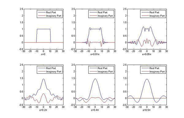
Actually, fractional Fourier transform is a rotation operation on the time frequency distribution. From the definition above, for α = 0, there will be no change after applying fractional Fourier transform, and for α = π/2, fractional Fourier transform becomes a Fourier transform, which rotates the time frequency distribution with π/2. For other value of α, fractional Fourier transform rotates the time frequency distribution according to α. The following figure shows the results of the fractional Fourier transform with different values of α.

Application

Fractional Fourier transform can be used in time frequency analysis and DSP. It is useful to filter noise, but with the condition that it does not overlap with the desired signal in the time–frequency domain. Consider the following example. We cannot apply a filter directly to eliminate the noise, but with the help of the fractional Fourier transform, we can rotate the signal (including the desired signal and noise) first. We then apply a specific filter, which will allow only the desired signal to pass. Thus the noise will be removed completely. Then we use the fractional Fourier transform again to rotate the signal back and we can get the desired signal.

Fractional Fourier transforms are also used to design optical systems and optimize holographic storage efficiency.

Thus, using just truncation in the time domain, or equivalently low-pass filters in the frequency domain, one can cut out any convex set in time–frequency space; just using time domain or frequency domain methods without fractional Fourier transforms only allow cutting out rectangles parallel to the axes.