
 | ||
In mathematics, the Bernoulli numbers Bn are a sequence of rational numbers with deep connections to number theory. The values of the first few Bernoulli numbers are
Contents
- Sum of powers
- Definitions
- Recursive definition
- Explicit definition
- Generating function
- Algorithmic description
- Efficient computation of Bernoulli numbers
- Different viewpoints and conventions
- Asymptotic analysis
- Taylor series of tan and tanh
- Use in topology
- Combinatorial definitions
- Connection with Worpitzky numbers
- Connection with Stirling numbers of the second kind
- Connection with Stirling numbers of the first kind
- Connection with Eulerian numbers
- Connection with Balmer series
- Representation of the second Bernoulli numbers
- A binary tree representation
- Asymptotic approximation
- Integral representation and continuation
- The relation to the Euler numbers and
- An algorithmic view the Seidel triangle
- A combinatorial view alternating permutations
- Related sequences
- Generalization to the odd index Bernoulli numbers
- A companion to the second Bernoulli numbers
- Arithmetical properties of the Bernoulli numbers
- The Kummer theorems
- p adic continuity
- Ramanujans congruences
- Von StaudtClausen theorem
- Why do the odd Bernoulli numbers vanish
- A restatement of the Riemann hypothesis
- Early history
- Reconstruction of Summae Potestatum
- Generalized Bernoulli numbers
- Values of the first Bernoulli numbers
- A subsequence of the Bernoulli number denominators
- References
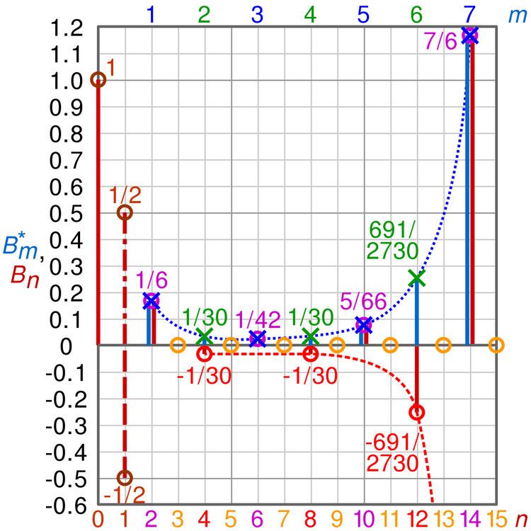
1 = ±1/2, B2 = 1/6, B3 = 0, B4 = −1/30, B5 = 0, B6 = 1/42, B7 = 0, B8 = −1/30.
The superscript ± is used by this article to designate the two sign conventions for Bernoulli numbers. They differ only in the sign of the n = 1 term:
n are the first Bernoulli numbers ( A027641 / A027642), and is the one prescribed by NIST. In this convention, B−
1 = −1/2.
n are the second Bernoulli numbers ( A164555 / A027642), which are also called the "original Bernoulli numbers". In this convention, B+
1 = +1/2.
Since Bn = 0 for all odd n > 1, and many formulas only involve even-index Bernoulli numbers, some authors write "Bn" to mean B2n. This article does not follow this notation.
The Bernoulli numbers appear in the Taylor series expansions of the tangent and hyperbolic tangent functions, in formulas for the sum of powers of the first positive integers, in the Euler–Maclaurin formula, and in expressions for certain values of the Riemann zeta function.
The Bernoulli numbers were discovered around the same time by the Swiss mathematician Jakob Bernoulli, after whom they are named, and independently by Japanese mathematician Seki Kōwa. Seki's discovery was posthumously published in 1712 in his work Katsuyo Sampo; Bernoulli's, also posthumously, in his Ars Conjectandi of 1713. Ada Lovelace's note G on the analytical engine from 1842 describes an algorithm for generating Bernoulli numbers with Babbage's machine. As a result, the Bernoulli numbers have the distinction of being the subject of the first published complex computer program.
Sum of powers
Bernoulli numbers feature prominently in the closed form expression of the sum of the mth powers of the first n positive integers. For m, n ≥ 0 define
This expression can always be rewritten as a polynomial in n of degree m + 1. The coefficients of these polynomials are related to the Bernoulli numbers by Bernoulli's formula:
where (m + 1
k) denotes the binomial coefficient.
For example, taking m to be 1 gives the triangular numbers 0, 1, 3, 6, … A000217.
Taking m to be 2 gives the square pyramidal numbers 0, 1, 5, 14, … A000330.
Some authors use the alternate convention for Bernoulli numbers and state Bernoulli's formula in this way:
Bernoulli's formula is sometimes called Faulhaber's formula after Johann Faulhaber who also found remarkable ways to calculate sums of powers.
Faulhaber's formula was generalized by V. Guo and J. Zeng to a q-analog (Guo & Zeng 2005).
Definitions
Many characterizations of the Bernoulli numbers have been found in the last 300 years, and each could be used to introduce these numbers. Here only four of the most useful ones are mentioned:
For the proof of the equivalence of the four approaches the reader is referred to mathematical expositions like (Ireland & Rosen 1990) or (Conway & Guy 1996).
Unfortunately in the literature the definition is given in two variants: Despite the fact that Bernoulli originally defined B+
1 = +1/2 (now known as "second Bernoulli numbers"), some authors chose B−
1 = −1/2 ("first Bernoulli numbers"). In order to prevent potential confusions both variants will be described here, side by side. Because these two definitions can be transformed simply by B+
n = (−1)n B−
n into the other, some formulae have this alternating (−1)n factor and others do not depending on the context. Some formulas appear simpler with the +1/2 convention, while others appear simpler with the −1/2 convention, hence there is no particular reason to consider either of these definitions to be the more "natural" one.
Recursive definition
The recursive equation is best introduced in a slightly more general form
This defines polynomials Bm in the variable n known as the Bernoulli polynomials. The recursion can also be viewed as defining rational numbers Bm(n) for all integers n ≥ 0, m ≥ 0. The expression 00 should be interpreted as 1 here. The first (−) and second (+) Bernoulli numbers now follow by setting n = 0 and n = 1 respectively.
where δ denotes the Kronecker delta. Whenever a confusion between the two kinds of definitions might arise it can be avoided by referring to the more general definition and by reintroducing the erased parameter: writing Bm(0) in the first case and Bm(1) in the second will unambiguously denote the value in question.
Explicit definition
Starting again with a slightly more general formula
The choices n = 0 and n = 1 lead to
In 1893 Louis Saalschütz listed a total of 38 explicit formulas for the Bernoulli numbers (Saalschütz 1893), usually giving some reference in the older literature.
Generating function
The general formula for the exponential generating function is
The choices n = 0 and n = 1 lead to
The (normal) generating function
is an asymptotic series. It contains the trigamma function ψ1.
Algorithmic description
Although the above recursive formula can be used for computation it is mainly used to establish the connection with the sum of powers because it is computationally expensive. However, both simple and high-end algorithms for computing Bernoulli numbers exist. Pointers to high-end algorithms are given the next section. A simple one is given in pseudocode below.
Efficient computation of Bernoulli numbers
In some applications it is useful to be able to compute the Bernoulli numbers B0 through Bp − 3 modulo p, where p is a prime; for example to test whether Vandiver's conjecture holds for p, or even just to determine whether p is an irregular prime. It is not feasible to carry out such a computation using the above recursive formulae, since at least (a constant multiple of) p2 arithmetic operations would be required. Fortunately, faster methods have been developed (Buhler et al. 2001) which require only O(p (log p)2) operations (see big O notation).
David Harvey (Harvey 2008) describes an algorithm for computing Bernoulli numbers by computing Bn modulo p for many small primes p, and then reconstructing Bn via the Chinese Remainder Theorem. Harvey writes that the asymptotic time complexity of this algorithm is O(n2 log(n)2 + ε) and claims that this implementation is significantly faster than implementations based on other methods. Using this implementation Harvey computed Bn for n = 108. Harvey's implementation has been included in SageMath since version 3.1. Prior to that, Bernd Kellner (Kellner 2002) computed Bn to full precision for n = 106 in December 2002 and Oleksandr Pavlyk (Pavlyk 2008) for n = 107 with Mathematica in April 2008.
Different viewpoints and conventions
The Bernoulli numbers can be regarded from four main viewpoints:
Each of these viewpoints leads to a set of more or less different conventions.
Associated sequence: 1/6, −1/30, 1/42, −1/30, …
This is the viewpoint of Jakob Bernoulli. (See the cutout from his Ars Conjectandi, first edition, 1713). The Bernoulli numbers are understood as numbers, recursive in nature, invented to solve a certain arithmetical problem, the summation of powers, which is the paradigmatic application of the Bernoulli numbers. These are also the numbers appearing in the Taylor series expansion of tan and tanh. It is misleading to call this viewpoint "archaic". For example, Jean-Pierre Serre uses it in his highly acclaimed book A Course in Arithmetic which is a standard textbook used at many universities today.
Associated sequence: 1, +1/2, 1/6, 0, …
This view focuses on the connection between Stirling numbers and Bernoulli numbers and arises naturally in the calculus of finite differences. In its most general and compact form this connection is summarized by the definition of the Stirling polynomials σn(x) (the definition of σ differs slightly from the corresponding Wikipedia article), formula (6.52) in Concrete Mathematics by Graham, Knuth and Patashnik.
In consequence B+
n = n! σn(1) for n ≥ 0.
Assuming the Bernoulli polynomials as already introduced the Bernoulli numbers can be defined in two different ways:
n = Bn(0). Associated sequence: 1, −1/2, 1/6, 0, …
n = Bn(1). Associated sequence: 1, +1/2, 1/6, 0, …
The two definitions differ only in the sign of B1. The choice B−
n = Bn(0) is the convention used in the Handbook of Mathematical Functions.
Associated sequence: 1, +1/2, 1/6, 0, …
Using this convention, the values of the Riemann zeta function satisfy nζ(1 − n) = −B+
n for all integers n ≥ 0. (See the paper of S. C. Woon; the expression nζ(1 − n) for n = 0 is to be understood as limx → 0 xζ(1 − x).)
Asymptotic analysis
Arguably the most important application of the Bernoulli number in mathematics is their use in the Euler–Maclaurin formula. Assuming that f is a sufficiently often differentiable function the Euler–Maclaurin formula can be written as
This formulation assumes the convention B−
1 = −1/2. Using the convention B+
1 = +1/2 the formula becomes
Here f(0) = f (i.e. the zeroth-order derivative of a f is just f). Moreover, let f(−1) denote an antiderivative of f. By the fundamental theorem of calculus,
Thus the last formula can be further simplified to the following succinct form of the Euler–Maclaurin formula
This form is for example the source for the important Euler–Maclaurin expansion of the zeta function
Here sk denotes the rising factorial power.
Bernoulli numbers are also frequently used in other kinds of asymptotic expansions. The following example is the classical Poincaré-type asymptotic expansion of the digamma function ψ.
Taylor series of tan and tanh
The Bernoulli numbers appear in the Taylor series expansion of the tangent and the hyperbolic tangent functions:
Use in topology
The Kervaire–Milnor formula for the order of the cyclic group of diffeomorphism classes of exotic (4n − 1)-spheres which bound parallelizable manifolds involves Bernoulli numbers. Let ESn be the number of such exotic spheres for n ≥ 2, then
The Hirzebruch signature theorem for the L genus of a smooth oriented closed manifold of dimension 4n also involves Bernoulli numbers.
Combinatorial definitions
The connection of the Bernoulli number to various kinds of combinatorial numbers is based on the classical theory of finite differences and on the combinatorial interpretation of the Bernoulli numbers as an instance of a fundamental combinatorial principle, the inclusion-exclusion principle.
Connection with Worpitzky numbers
The definition to proceed with was developed by Julius Worpitzky in 1883. Besides elementary arithmetic only the factorial function n! and the power function km is employed. The signless Worpitzky numbers are defined as
They can also be expressed through the Stirling numbers of the second kind
A Bernoulli number is then introduced as an inclusion–exclusion sum of Worpitzky numbers weighted by the harmonic sequence 1, 1/2, 1/3, …
This representation has B+
1 = +1/2.
Consider the sequence sn, n ≥ 0. From Worpitzky's numbers A028246, A163626 applied to s0, s0, s1, s0, s1, s2, s0, s1, s2, s3, … is identical to the Akiyama–Tanigawa transform applied to sn (see Connection with Stirling numbers of the first kind). This can be seen via the table:
The first row represents s0, s1, s2, s3, s4.
Hence for the second fractional Euler numbers A198631 (n) / A006519 (n + 1):
E0 = 1E1 = 1 − 1/2E2 = 1 − 3/2 + 2/4E3 = 1 − 7/2 + 12/4 − 6/8E4 = 1 − 15/2 + 50/4 − 60/8 + 24/16E5 = 1 − 31/2 + 180/4 − 390/8 + 360/16 − 120/32E6 = 1 − 63/2 + 602/4 − 2100/8 + 3360/16 − 2520/32 + 720/64A second formula representing the Bernoulli numbers by the Worpitzky numbers is for n ≥ 1
The simplified second Worpitzky's representation of the second Bernoulli numbers is:
A164555 (n + 1) / A027642(n + 1) = n + 1/2n + 2 − 2 × A198631(n) / A006519(n + 1)
which links the second Bernoulli numbers to the second fractional Euler numbers. The beginning is:
1/2, 1/6, 0, −1/30, 0, 1/42, … = (1/2, 1/3, 3/14, 2/15, 5/62, 1/21, …) × (1, 1/2, 0, −1/4, 0, 1/2, …)The numerators of the first parentheses are A111701 (see Connection with Stirling numbers of the first kind).
Connection with Stirling numbers of the second kind
If S(k,m) denotes Stirling numbers of the second kind then one has:
where jm denotes the falling factorial.
If one defines the Bernoulli polynomials Bk(j) as:
where Bk for k = 0, 1, 2,… are the Bernoulli numbers.
Then after the following property of binomial coefficient:
one has,
One also has following for Bernoulli polynomials,
The coefficient of j in (j
m + 1) is (−1)m/m + 1.
Comparing the coefficient of j in the two expressions of Bernoulli polynomials, one has:
(resulting in B1 = +1/2) which is an explicit formula for Bernoulli numbers and can be used to prove Von-Staudt Clausen theorem.
Connection with Stirling numbers of the first kind
The two main formulas relating the unsigned Stirling numbers of the first kind [n
m] to the Bernoulli numbers (with B1 = +1/2) are
and the inversion of this sum (for n ≥ 0, m ≥ 0)
Here the number An,m are the rational Akiyama–Tanigawa numbers, the first few of which are displayed in the following table.
The Akiyama–Tanigawa numbers satisfy a simple recurrence relation which can be exploited to iteratively compute the Bernoulli numbers. This leads to the algorithm shown in the section 'algorithmic description' above. See A051714/ A051715.
An autosequence is a sequence which has its inverse binomial transform equal to the signed sequence. If the main diagonal is zeroes = A000004, the autosequence is of the first kind. Example: A000045, the Fibonacci numbers. If the main diagonal is the first upper diagonal multiplied by 2, it is of the second kind. Example: A164555/ A027642, the second Bernoulli numbers (see A190339). The Akiyama–Tanigawa transform applied to 2−n = 1/ A000079 leads to A198631 (n) / A06519 (n + 1). Hence:
See A209308 and A227577. A198631 (n) / A006519 (n + 1) are the second (fractional) Euler numbers and an autosequence of the second kind.
( A164555 (n + 2)/ A027642 (n + 2) = 1/6, 0, −1/30, 0, 1/42, …) × ( 2n + 3 − 2/n + 2 = 3, 14/3, 15/2, 62/5, 21, …) = A198631 (n + 1)/ A006519 (n + 2) = 1/2, 0, −1/4, 0, 1/2, ….Also valuable for A027641 / A027642 (see Connection with Worpitzky numbers).
Connection with Eulerian numbers
There are formulas connecting Eulerian numbers ⟨n
m⟩ to Bernoulli numbers:
Both formulae are valid for n ≥ 0 if B1 is set to 1/2. If B1 is set to −1/2 they are valid only for n ≥ 1 and n ≥ 2 respectively.
Connection with Balmer series
A link between Bernoulli numbers and Balmer series can be seen in sequence A191567.
Representation of the second Bernoulli numbers
See A191302. The numbers are not reduced. Then the columns are easy to find, the denominators being A190339.
B0 = 1 (= 2/2)B1 = 1/2B2 = 1/2 − 2/6B3 = 1/2 − 3/6B4 = 1/2 − 4/6 + 2/15B5 = 1/2 − 5/6 + 5/15B6 = 1/2 − 6/6 + 9/15 − 8/105B7 = 1/2 − 7/6 + 14/15 − 28/105A binary tree representation
The Stirling polynomials σn(x) are related to the Bernoulli numbers by Bn = n!σn(1). S. C. Woon (Woon 1997) described an algorithm to compute σn(1) as a binary tree:
Woon's recursive algorithm (for n ≥ 1) starts by assigning to the root node N = [1,2]. Given a node N = [a1, a2, …, ak] of the tree, the left child of the node is L(N) = [−a1, a2 + 1, a3, …, ak] and the right child R(N) = [a1, 2, a2, …, ak]. A node N = [a1, a2, …, ak] is written as ±[a2, …, ak] in the initial part of the tree represented above with ± denoting the sign of a1.
Given a node N the factorial of N is defined as
Restricted to the nodes N of a fixed tree-level n the sum of 1/N! is σn(1), thus
For example:
B1 = 1!(1/2!)B2 = 2!(−1/3! + 1/2!2!)B3 = 3!(1/4! − 1/2!3! − 1/3!2! + 1/2!2!2!)Asymptotic approximation
The Bernoulli numbers can be expressed in terms of the Riemann zeta function as
It then follows from the Stirling formula that, as n goes to infinity,
Including more terms from the zeta series yields a better approximation, as does factoring in the asymptotic series in Stirling's approximation.
Integral representation and continuation
The integral
has as special values b(2n) = B2n for n > 0.
For example, b(3) = 3/2ζ(3)Π−3Ι and b(5) = −15/2ζ(5)Π−5Ι. Here ζ(n) denotes the Riemann zeta function and Ι the imaginary unit. Already Leonhard Euler (Opera Omnia, Ser. 1, Vol. 10, p. 351) considered these numbers and calculated
The relation to the Euler numbers and π
The Euler numbers are a sequence of integers intimately connected with the Bernoulli numbers. Comparing the asymptotic expansions of the Bernoulli and the Euler numbers shows that the Euler numbers E2n are in magnitude approximately 2/π(42n − 22n) times larger than the Bernoulli numbers B2n. In consequence:
This asymptotic equation reveals that π lies in the common root of both the Bernoulli and the Euler numbers. In fact π could be computed from these rational approximations.
Bernoulli numbers can be expressed through the Euler numbers and vice versa. Since, for odd n, Bn = En = 0 (with the exception B1), it suffices to consider the case when n is even.
These conversion formulas express an inverse relation between the Bernoulli and the Euler numbers. But more important, there is a deep arithmetic root common to both kinds of numbers, which can be expressed through a more fundamental sequence of numbers, also closely tied to π. These numbers are defined for n > 1 as
and S1 = 1 by convention (Elkies 2003). The magic of these numbers lies in the fact that they turn out to be rational numbers. This was first proved by Leonhard Euler in a landmark paper (Euler 1735) ‘De summis serierum reciprocarum’ (On the sums of series of reciprocals) and has fascinated mathematicians ever since. The first few of these numbers are
These are the coefficients in the expansion of sec x + tan x.
The Bernoulli numbers and Euler numbers are best understood as special views of these numbers, selected from the sequence Sn and scaled for use in special applications.
The expression [n even] has the value 1 if n is even and 0 otherwise (Iverson bracket).
These identities show that the quotient of Bernoulli and Euler numbers at the beginning of this section is just the special case of Rn = 2Sn/Sn + 1 when n is even. The Rn are rational approximations to π and two successive terms always enclose the true value of π. Beginning with n = 1 the sequence starts ( A132049 / A132050):
These rational numbers also appear in the last paragraph of Euler's paper cited above.
Consider the Akiyama–Tanigawa transform for the sequence A046978 (n + 2) / A016116 (n + 1):
From the second, the numerators of the first column are the denominators of Euler's formula. The first column is −1/2 × A163982.
An algorithmic view: the Seidel triangle
The sequence Sn has another unexpected yet important property: The denominators of Sn divide the factorial (n − 1)!. In other words: the numbers Tn = Sn(n − 1)!, sometimes called Euler zigzag numbers, are integers.
Thus the above representations of the Bernoulli and Euler numbers can be rewritten in terms of this sequence as
These identities make it easy to compute the Bernoulli and Euler numbers: the Euler numbers En are given immediately by T2n + 1 and the Bernoulli numbers B2n are obtained from T2n by some easy shifting, avoiding rational arithmetic.
What remains is to find a convenient way to compute the numbers Tn. However, already in 1877 Philipp Ludwig von Seidel (Seidel 1877) published an ingenious algorithm which makes it extremely simple to calculate Tn.
- Start by putting 1 in row 0 and let k denote the number of the row currently being filled
- If k is odd, then put the number on the left end of the row k − 1 in the first position of the row k, and fill the row from the left to the right, with every entry being the sum of the number to the left and the number to the upper
- At the end of the row duplicate the last number.
- If k is even, proceed similar in the other direction.
Seidel's algorithm is in fact much more general (see the exposition of Dominique Dumont (Dumont 1981)) and was rediscovered several times thereafter.
Similar to Seidel's approach D. E. Knuth and T. J. Buckholtz (Knuth & Buckholtz 1967) gave a recurrence equation for the numbers T2n and recommended this method for computing B2n and E2n ‘on electronic computers using only simple operations on integers’.
V. I. Arnold rediscovered Seidel's algorithm in (Arnold 1991) and later Millar, Sloane and Young popularized Seidel's algorithm under the name boustrophedon transform.
Triangular form:
Only A000657, with one 1, and A214267, with two 1s, are in the OEIS.
Distribution with a supplementary 1 and one 0 in the following rows:
This is A239005, a signed version of A008280. The main andiagonal is A122045. The main diagonal is A155585. The central column is A099023. Row sums: 1, 1, −2, −5, 16, 61…. See A163747. See the array beginning with 1, 1, 0, −2, 0, 16, 0 below.
The Akiyama–Tanigawa algorithm applied to A046978 (n + 1) / A016116(n) yields:
1. The first column is A122045. Its binomial transform leads to:
The first row of this array is A155585. The absolute values of the increasing antidiagonals are A008280. The sum of the antidiagonals is − A163747 (n + 1).
2. The second column is 1 1 −1 −5 5 61 −61 −1385 1385…. Its binomial transform yields:
The first row of this array is 1 2 2 −4 −16 32 272 544 −7936 15872 353792 −707584…. The absolute values of the second bisection are the double of the absolute values of the first bisection.
Consider the Akiyama-Tanigawa algorithm applied to A046978 (n) / ( A158780 (n + 1) = abs( A117575 (n)) + 1 = 1, 2, 2, 3/2, 1, 3/4, 3/4, 7/8, 1, 17/16, 17/16, 33/32….
The first column whose the absolute values are A000111 could be the numerator of a trigonometric function.
A163747 is an autosequence of the first kind (the main diagonal is A000004). The corresponding array is:
The first two upper diagonals are −1 3 −24 402… = (−1)n + 1 × A002832. The sum of the antidiagonals is 0 −2 0 10… = 2 × A122045(n + 1).
− A163982 is an autosequence of the second kind, like for instance A164555 / A027642. Hence the array:
The main diagonal, here 2 −2 8 −92…, is the double of the first upper one, here A099023. The sum of the antidiagonals is 2 0 −4 0… = 2 × A155585(n + 1). Note that A163747 − A163982 = 2 × A122045.
A combinatorial view: alternating permutations
Around 1880, three years after the publication of Seidel's algorithm, Désiré André proved a now classic result of combinatorial analysis (André 1879) & (André 1881). Looking at the first terms of the Taylor expansion of the trigonometric functions tan x and sec x André made a startling discovery.
The coefficients are the Euler numbers of odd and even index, respectively. In consequence the ordinary expansion of tan x + sec x has as coefficients the rational numbers Sn.
André then succeeded by means of a recurrence argument to show that the alternating permutations of odd size are enumerated by the Euler numbers of odd index (also called tangent numbers) and the alternating permutations of even size by the Euler numbers of even index (also called secant numbers).
Related sequences
The arithmetic mean of the first and the second Bernoulli numbers are the associate Bernoulli numbers: B0 = 1, B1 = 0, B2 = 1/6, B3 = 0, B4 = −1/30, A176327 / A027642. Via the second row of its inverse Akiyama–Tanigawa transform A177427, they lead to Balmer series A061037 / A061038.
The Akiyama–Tanigawa algorithm applied to A060819 (n + 4) / A145979 (n) leads to the Bernoulli numbers A027641 / A027642, A164555 / A027642, or A176327 A176289 without B1, named intrinsic Bernoulli numbers Bi(n).
Hence another link between the intrinsic Bernoulli numbers and the Balmer series via A145979 (n).
A145979 (n − 2) = 0, 2, 1, 6,… is a permutation of the non-negative numbers.
The terms of the first row are 1/2 + 1/n + 2.
Euler A198631 (n) / A006519 (n + 1) without the second term (1/2) are the fractional intrinsic Euler numbers Ei(n) = 1, 0, −1/4, 0, 1/2, 0, −17/8, 0, … The corresponding Akiyama transform is:
The first line is Eu(n). Eu(n) preceded by a zero is an autosequence of the first kind. It is linked to the Oresme numbers. The numerators of the second line are A069834 preceded by 0. The difference table is:
Generalization to the odd-index Bernoulli numbers
1, 1/2, 1/6, 3/56, 1/30, 25/992, 1/42, 427/16256, 1/30, 12465/261632, 5/66, 555731/4102256, 691/2730, 35135945/67100672, 7/6, 2990414715/1073709056,… ( A193472/ A193473)This is ez(n − 1)n!/4n − 2n where ez(n) is the nth coefficient of sec t + tan t ( A000111/ A000142).
A companion to the second Bernoulli numbers
See A190339. The following fractional numbers are an autosequence of the first kind.
A191754 / A192366 = 0, 1/2, 1/2, 1/3, 1/6, 1/15, 1/30, 1/35, 1/70, –1/105, –1/210, 41/1155, 41/2310, –589/5005, −589/10010 …Apply T(n + 1, k) = 2T(n, k + 1) − T(n,k) to T(0,k) = A191754 (k)/ A192366(k):
The rows are alternatively autosequences of the first and of the second kind. The second row is A164555/ A027642. For the third row, see A051716.
The first column is 0, 1, 0, −1/3, 0, 7/15, 0, −31/21, 0, 127/105, 0, −511/33,… from Mersenne primes, see A141459. For the second column see A140252.
Consider the triangle A097805 (n + 1) = Fiba(n) =
This is Pascal's triangle A0007318 bordered by zeroes. The antidiagonals' sums are A000045, the Fibonacci numbers. Two elementary transforms yield the array ASPEC0, a companion to ASPEC in A191302.
Multiplying the SBD array in A191302 by ASPEC0, we have by row sums A191754/ A192366:
This triangle is unreduced.
Arithmetical properties of the Bernoulli numbers
The Bernoulli numbers can be expressed in terms of the Riemann zeta function as Bn = −nζ(1 − n) for integers n ≥ 0 provided for n = 0 and n = 1 the expression −nζ(1 − n) is understood as the limiting value and the convention B1 = 1/2 is used. This intimately relates them to the values of the zeta function at negative integers. As such, they could be expected to have and do have deep arithmetical properties. For example, the Agoh–Giuga conjecture postulates that p is a prime number if and only if pBp − 1 is congruent to −1 modulo p. Divisibility properties of the Bernoulli numbers are related to the ideal class groups of cyclotomic fields by a theorem of Kummer and its strengthening in the Herbrand-Ribet theorem, and to class numbers of real quadratic fields by Ankeny–Artin–Chowla.
The Kummer theorems
The Bernoulli numbers are related to Fermat's last theorem (FLT) by Kummer's theorem (Kummer 1850), which says:
If the odd prime p does not divide any of the numerators of the Bernoulli numbers B2, B4, …, Bp − 3 then xp + yp + zp = 0 has no solutions in nonzero integers.Prime numbers with this property are called regular primes. Another classical result of Kummer (Kummer 1851) are the following congruences.
Let p be an odd prime and b an even number such that p − 1 does not divide b. Then for any non-negative integer kA generalization of these congruences goes by the name of p-adic continuity.
p-adic continuity
If b, m and n are positive integers such that m and n are not divisible by p − 1 and m ≡ n mod pb − 1 (p − 1), then
Since Bn = −nζ(1 − n), this can also be written
where u = 1 − m and v = 1 − n, so that u and v are nonpositive and not congruent to 1 modulo p − 1. This tells us that the Riemann zeta function, with 1 − p−s taken out of the Euler product formula, is continuous in the p-adic numbers on odd negative integers congruent modulo p − 1 to a particular a ≢ 1 mod (p − 1), and so can be extended to a continuous function ζp(s) for all p-adic integers ℤp, the p-adic zeta function.
Ramanujan's congruences
The following relations, due to Ramanujan, provide a method for calculating Bernoulli numbers that is more efficient than the one given by their original recursive definition:
Von Staudt–Clausen theorem
The von Staudt–Clausen theorem was given by Karl Georg Christian von Staudt (von Staudt 1840) and Thomas Clausen (Clausen 1840) independently in 1840. The theorem states that for every n > 0,
is an integer. The sum extends over all primes p for which p − 1 divides 2n.
A consequence of this is that the denominator of B2n is given by the product of all primes p for which p − 1 divides 2n. In particular, these denominators are square-free and divisible by 6.
Why do the odd Bernoulli numbers vanish?
The sum
can be evaluated for negative values of the index n. Doing so will show that it is an odd function for even values of k, which implies that the sum has only terms of odd index. This and the formula for the Bernoulli sum imply that B2k + 1 − m is 0 for m even and 2k + 1 − m > 1; and that the term for B1 is cancelled by the subtraction. The von Staudt–Clausen theorem combined with Worpitzky's representation also gives a combinatorial answer to this question (valid for n > 1).
From the von Staudt–Clausen theorem it is known that for odd n > 1 the number 2Bn is an integer. This seems trivial if one knows beforehand that the integer in question is zero. However, by applying Worpitzky's representation one gets
as a sum of integers, which is not trivial. Here a combinatorial fact comes to surface which explains the vanishing of the Bernoulli numbers at odd index. Let Sn,m be the number of surjective maps from {1, 2, …, n} to {1, 2, …, m}, then Sn,m = m!{n
m}. The last equation can only hold if
This equation can be proved by induction. The first two examples of this equation are
n = 4: 2 + 8 = 7 + 3,n = 6: 2 + 120 + 144 = 31 + 195 + 40.Thus the Bernoulli numbers vanish at odd index because some non-obvious combinatorial identities are embodied in the Bernoulli numbers.
A restatement of the Riemann hypothesis
The connection between the Bernoulli numbers and the Riemann zeta function is strong enough to provide an alternate formulation of the Riemann hypothesis (RH) which uses only the Bernoulli number. In fact Marcel Riesz (Riesz 1916) proved that the RH is equivalent to the following assertion:
For every ε > 1/4 there exists a constant Cε > 0 (depending on ε) such that | R(x) | < Cεxε as x → ∞.Here R(x) is the Riesz function
nk denotes the rising factorial power in the notation of D. E. Knuth. The numbers βn = Bn/n occur frequently in the study of the zeta function and are significant because βn is a p-integer for primes p where p − 1 does not divide n. The βn are called divided Bernoulli numbers.
Early history
The Bernoulli numbers are rooted in the early history of the computation of sums of integer powers, which have been of interest to mathematicians since antiquity.
Methods to calculate the sum of the first n positive integers, the sum of the squares and of the cubes of the first n positive integers were known, but there were no real 'formulas', only descriptions given entirely in words. Among the great mathematicians of antiquity which considered this problem were: Pythagoras (c. 572–497 BCE, Greece), Archimedes (287–212 BCE, Italy), Aryabhata (b. 476, India), Abu Bakr al-Karaji (d. 1019, Persia) and Abu Ali al-Hasan ibn al-Hasan ibn al-Haytham (965–1039, Iraq).
During the late sixteenth and early seventeenth centuries mathematicians made significant progress. In the West Thomas Harriot (1560–1621) of England, Johann Faulhaber (1580–1635) of Germany, Pierre de Fermat (1601–1665) and fellow French mathematician Blaise Pascal (1623–1662) all played important roles.
Thomas Harriot seems to have been the first to derive and write formulas for sums of powers using symbolic notation, but even he calculated only up to the sum of the fourth powers. Johann Faulhaber gave formulas for sums of powers up to the 17th power in his 1631 Academia Algebrae, far higher than anyone before him, but he did not give a general formula.
Blaise Pascal in 1654 proved Pascal's identity relating the sums of the pth powers of the first n positive integers for p = 0, 1, 2, …, k.
The Swiss mathematician Jakob Bernoulli (1654–1705) was the first to realize the existence of a single sequence of constants B0, B1, B2,… which provide a uniform formula for all sums of powers (Knuth 1993).
The joy Bernoulli experienced when he hit upon the pattern needed to compute quickly and easily the coefficients of his formula for the sum of the cth powers for any positive integer c can be seen from his comment. He wrote:
"With the help of this table, it took me less than half of a quarter of an hour to find that the tenth powers of the first 1000 numbers being added together will yield the sum 91,409,924,241,424,243,424,241,924,242,500."Bernoulli's result was published posthumously in Ars Conjectandi in 1713. Seki Kōwa independently discovered the Bernoulli numbers and his result was published a year earlier, also posthumously, in 1712. However, Seki did not present his method as a formula based on a sequence of constants.
Bernoulli's formula for sums of powers is the most useful and generalizable formulation to date. The coefficients in Bernoulli's formula are now called Bernoulli numbers, following a suggestion of Abraham de Moivre.
Bernoulli's formula is sometimes called Faulhaber's formula after Johann Faulhaber who found remarkable ways to calculate sum of powers but never stated Bernoulli's formula. To call Bernoulli's formula Faulhaber's formula does injustice to Bernoulli and simultaneously hides the genius of Faulhaber as Faulhaber's formula is in fact more efficient than Bernoulli's formula. According to Knuth (Knuth 1993) a rigorous proof of Faulhaber's formula was first published by Carl Jacobi in 1834 (Jacobi 1834). E. Knuth's in-depth study of Faulhaber's formula concludes:
"Faulhaber never discovered the Bernoulli numbers; i.e., he never realized that a single sequence of constants B0, B1, B2, … would provide a uniformfor all sums of powers. He never mentioned, for example, the fact that almost half of the coefficients turned out to be zero after he had converted his formulas for ∑ nm from polynomials in N to polynomials in n." (Knuth 1993, p. 14)Reconstruction of "Summae Potestatum"
The Bernoulli numbers were introduced by Jakob Bernoulli in the book Ars Conjectandi published posthumously in 1713 page 97. The main formula can be seen in the second half of the corresponding facsimile. The constant coefficients denoted A, B, C and D by Bernoulli are mapped to the notation which is now prevalent as A = B2, B = B4, C = B6, D = B8. The expression c·c−1·c−2·c−3 means c·(c−1)·(c−2)·(c−3) – the small dots are used as grouping symbols. Using today's terminology these expressions are falling factorial powers ck. The factorial notation k! as a shortcut for 1 × 2 × … × k was not introduced until 100 years later. The integral symbol on the left hand side goes back to Gottfried Wilhelm Leibniz in 1675 who used it as a long letter S for "summa" (sum). (The Mathematics Genealogy Project shows Leibniz as the doctoral adviser of Jakob Bernoulli. See also the Earliest Uses of Symbols of Calculus.) The letter n on the left hand side is not an index of summation but gives the upper limit of the range of summation which is to be understood as 1, 2, …, n. Putting things together, for positive c, today a mathematician is likely to write Bernoulli's formula as:
In fact this formula imperatively suggests to set B1 = 1/2 when switching from the so-called 'archaic' enumeration which uses only the even indices 2, 4, 6… to the modern form (more on different conventions in the next paragraph). Most striking in this context is the fact that the falling factorial ck−1 has for k = 0 the value 1/c + 1. Thus Bernoulli's formula can and has to be written
if B1 stands for the value Bernoulli himself has given to the coefficient at that position.
Generalized Bernoulli numbers
The generalized Bernoulli numbers are certain algebraic numbers, defined similarly to the Bernoulli numbers, that are related to special values of Dirichlet L-functions in the same way that Bernoulli numbers are related to special values of the Riemann zeta function.
Let χ be a Dirichlet character modulo f. The generalized Bernoulli numbers attached to χ are defined by
Apart from the exceptional B1,1 = 1/2, we have, for any Dirichlet character χ, that Bk,χ = 0 if χ(−1) ≠ (−1)k.
Generalizing the relation between Bernoulli numbers and values of the Riemann zeta function at non-positive integers, one has the for all integers k ≥ 1:
where L(s,χ) is the Dirichlet L-function of χ.
Values of the first Bernoulli numbers
Bn = 0 for all odd n other than 1. For even n, Bn is negative if n is divisible by 4 and positive otherwise. The first few non-zero Bernoulli numbers are:
From 6, the denominators are multiples of the sequence of period 2: {6,30} A165734. From 2, the denominators are of the form 4k + 2.
A subsequence of the Bernoulli number denominators
A219196 = A027642( A131577) =
1, 2, 6, 30, 30, 510, 510, 510, 510, 131070, 131070, 131070, 131070, 131070, 131070, 131070, 131070, 8589934590, 8589934590, 8589934590, 8589934590, 8589934590, 8589934590, 8589934590, 8589934590, 8589934590, 8589934590, 8589934590, 8589934590, 8589934590, 8589934590, 8589934590, 8589934590, 8589934590, 8589934590, 8589934590, 8589934590