
 | ||
In mathematics, the Riesz function is an entire function defined by Marcel Riesz in connection with the Riemann hypothesis, by means of the power series
Contents
- Riesz criterion
- Mellin transform of the Riesz function
- Calculation of the Riesz function
- Appearance of the Riesz function
- References
If we set
then F may be defined as
The values of ζ(2k) approach one for increasing k, and comparing the series for the Riesz function with that for
Riesz criterion
It can be shown that
for any exponent e larger than 1/2, where this is big O notation; taking values both positive and negative. Riesz showed that the Riemann hypothesis is equivalent to the claim that the above is true for any e larger than 1/4. In the same paper, he added a slightly pessimistic note too: «Je ne sais pas encore decider si cette condition facilitera la vérification de l'hypothèse».
Mellin transform of the Riesz function
The Riesz function is related to the Riemann zeta function via its Mellin transform. If we take
we see that if
converges, whereas from the growth condition we have that if
converges. Putting this together, we see the Mellin transform of the Riesz function is defined on the strip
From the inverse Mellin transform, we now get an expression for the Riesz function, as
where c is between minus one and minus one-half. If the Riemann hypothesis is true, we can move the line of integration to any value less than minus one-fourth, and hence we get the equivalence between the fourth-root rate of growth for the Riesz function and the Riemann hypothesis.
J. garcia (see references) gave the integral representation of
Calculation of the Riesz function
The Maclaurin series coefficients of F increase in absolute value until they reach their maximum at the 40th term of -1.753×10¹⁷. By the 109th term they have dropped below one in absolute value. Taking the first 1000 terms suffices to give a very accurate value for
Another approach is to use acceleration of convergence. We have
Since ζ(2k) approaches one as k grows larger, the terms of this series approach
Using Kummer's method for accelerating convergence gives
with an improved rate of convergence.
Continuing this process leads to a new series for the Riesz function with much better convergence properties:
Here μ is the Möbius mu function, and the rearrangement of terms is justified by absolute convergence. We may now apply Kummer's method again, and write
the terms of which eventually decrease as the inverse fourth power of n.
The above series are absolutely convergent everywhere, and hence may be differentiated term by term, leading to the following expression for the derivative of the Riesz function:
which may be rearranged as
Marek Wolf in assuming the Riemann Hypothesis has shown that for large x:
where
Appearance of the Riesz function
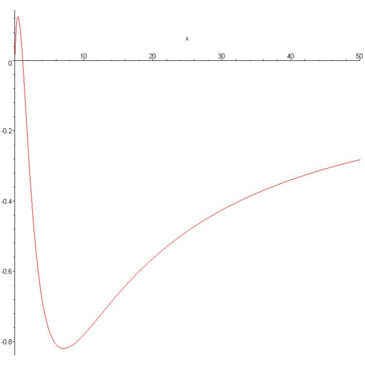
A plot for the range 0 to 50 is given above. So far as it goes, it does not indicate very rapid growth and perhaps bodes well for the truth of the Riemann hypothesis.