
 | ||
In mathematics, the Riemann hypothesis is a conjecture that the Riemann zeta function has its zeros only at the negative even integers and complex numbers with real part 1/2. It was proposed by Bernhard Riemann (1859), after whom it is named. The name is also used for some closely related analogues, such as the Riemann hypothesis for curves over finite fields.
Contents
- Riemann zeta function
- Origin
- Consequences
- Distribution of prime numbers
- Growth of arithmetic functions
- Lindelf hypothesis and growth of the zeta function
- Large prime gap conjecture
- Criteria equivalent to the Riemann hypothesis
- Consequences of the generalized Riemann hypothesis
- Excluded middle
- Littlewoods theorem
- Gausss class number conjecture
- Growth of Eulers totient
- Dirichlet L series and other number fields
- Function fields and zeta functions of varieties over finite fields
- Arithmetic zeta functions of arithmetic schemes and their L factors
- Selberg zeta functions
- Ihara zeta functions
- Montgomerys pair correlation conjecture
- Other zeta functions
- Attempted proofs
- Operator theory
- LeeYang theorem
- Turns result
- Noncommutative geometry
- Hilbert spaces of entire functions
- Quasicrystals
- Arithmetic zeta functions of models of elliptic curves over number fields
- Multiple zeta functions
- Number of zeros
- Theorem of Hadamard and de la Valle Poussin
- Zero free regions
- Zeros on the critical line
- HardyLittlewood conjectures
- Selbergs zeta function conjecture
- Numerical calculations
- Gram points
- Arguments for and against the Riemann hypothesis
- References
The Riemann hypothesis implies results about the distribution of prime numbers. Along with suitable generalizations, some mathematicians consider it the most important unresolved problem in pure mathematics (Bombieri 2000). The Riemann hypothesis, along with Goldbach's conjecture, is part of Hilbert's eighth problem in David Hilbert's list of 23 unsolved problems; it is also one of the Clay Mathematics Institute's Millennium Prize Problems.
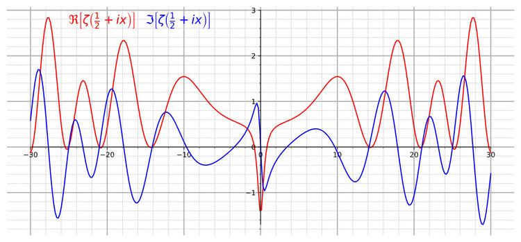
The Riemann zeta function ζ(s) is a function whose argument s may be any complex number other than 1, and whose values are also complex. It has zeros at the negative even integers; that is, ζ(s) = 0 when s is one of −2, −4, −6, .... These are called its trivial zeros. However, the negative even integers are not the only values for which the zeta function is zero. The other ones are called non-trivial zeros. The Riemann hypothesis is concerned with the locations of these non-trivial zeros, and states that:
The real part of every non-trivial zero of the Riemann zeta function is 1/2.Thus, if the hypothesis is correct, all the non-trivial zeros lie on the critical line consisting of the complex numbers 1/2 + i t, where t is a real number and i is the imaginary unit.
There are several nontechnical books on the Riemann hypothesis, such as Derbyshire (2003), Rockmore (2005), (Sabbagh 2003a, 2003b), du Sautoy (2003). The books Edwards (1974), Patterson (1988), Borwein et al. (2008) and Mazur & Stein (2015) give mathematical introductions, while Titchmarsh (1986), Ivić (1985) and Karatsuba & Voronin (1992) are advanced monographs. Furthermore, the book Open Problems in Mathematics, edited by John Forbes Nash Jr. and Michael Th. Rassias, features an extensive essay on the Riemann hypothesis by Alain Connes.
Riemann zeta function
The Riemann zeta function is defined for complex s with real part greater than 1 by the absolutely convergent infinite series
Leonhard Euler (who died 40 years before Riemann was born) showed that this series equals the Euler product
where the infinite product extends over all prime numbers p, and again converges for complex s with real part greater than 1. The convergence of the Euler product shows that ζ(s) has no zeros in this region, as none of the factors have zeros.
The Riemann hypothesis discusses zeros outside the region of convergence of this series and Euler product. To make sense of the hypothesis, it is necessary to analytically continue the function to give it a definition that is valid for all complex s. This can be done by expressing it in terms of the Dirichlet eta function as follows. If the real part of s is greater than one, then the zeta function satisfies
However, the series on the right converges not just when the real part of s is greater than one, but more generally whenever s has positive real part. Thus, this alternative series extends the zeta function from Re(s) > 1 to the larger domain Re(s) > 0, excluding the zeros
In the strip 0 < Re(s) < 1 the zeta function satisfies the functional equation
One may then define ζ(s) for all remaining nonzero complex numbers s by assuming that this equation holds outside the strip as well, and letting ζ(s) equal the right-hand side of the equation whenever s has non-positive real part. If s is a negative even integer then ζ(s) = 0 because the factor sin(πs/2) vanishes; these are the trivial zeros of the zeta function. (If s is a positive even integer this argument does not apply because the zeros of the sine function are cancelled by the poles of the gamma function as it takes negative integer arguments.) The value ζ(0) = −1/2 is not determined by the functional equation, but is the limiting value of ζ(s) as s approaches zero. The functional equation also implies that the zeta function has no zeros with negative real part other than the trivial zeros, so all non-trivial zeros lie in the critical strip where s has real part between 0 and 1.
Origin
"…es ist sehr wahrscheinlich, dass alle Wurzeln reell sind. Hiervon wäre allerdings ein strenger Beweis zu wünschen; ich habe indess die Aufsuchung desselben nach einigen flüchtigen vergeblichen Versuchen vorläufig bei Seite gelassen, da er für den nächsten Zweck meiner Untersuchung entbehrlich schien."
("…it is very probable that all roots are real. Of course one would wish for a rigorous proof here; I have for the time being, after some fleeting vain attempts, provisionally put aside the search for this, as it appears dispensable for the immediate objective of my investigation.")
Riemann's original motivation for studying the zeta function and its zeros was their occurrence in his explicit formula for the number of primes π(x) less than a given number x, which he published in his 1859 paper "On the Number of Primes Less Than a Given Magnitude". His formula was given in terms of the related function
which counts the primes and prime powers up to x, counting a prime power pn as 1/n of a prime. The number of primes can be recovered from this function by, using the Möbius inversion formula
where μ is the Möbius function. Riemann's formula is then
where the sum is over the nontrivial zeros of the zeta function and where Π0 is a slightly modified version of Π that replaces its value at its points of discontinuity by the average of its upper and lower limits:
The summation in Riemann's formula is not absolutely convergent, but may be evaluated by taking the zeros ρ in order of the absolute value of their imaginary part. The function Li occurring in the first term is the (unoffset) logarithmic integral function given by the Cauchy principal value of the divergent integral
The terms Li(xρ) involving the zeros of the zeta function need some care in their definition as Li has branch points at 0 and 1, and are defined (for x > 1) by analytic continuation in the complex variable ρ in the region Re(ρ) > 0, i.e. they should be considered as Ei(ρ ln x). The other terms also correspond to zeros: the dominant term Li(x) comes from the pole at s = 1, considered as a zero of multiplicity −1, and the remaining small terms come from the trivial zeros. For some graphs of the sums of the first few terms of this series see Riesel & Göhl (1970) or Zagier (1977).
This formula says that the zeros of the Riemann zeta function control the oscillations of primes around their "expected" positions. Riemann knew that the non-trivial zeros of the zeta function were symmetrically distributed about the line s = 1/2 + it, and he knew that all of its non-trivial zeros must lie in the range 0 ≤ Re(s) ≤ 1. He checked that a few of the zeros lay on the critical line with real part 1/2 and suggested that they all do; this is the Riemann hypothesis.
Consequences
The practical uses of the Riemann hypothesis include many propositions known true under the Riemann hypothesis, and some that can be shown equivalent to the Riemann hypothesis.
Distribution of prime numbers
Riemann's explicit formula for the number of primes less than a given number in terms of a sum over the zeros of the Riemann zeta function says that the magnitude of the oscillations of primes around their expected position is controlled by the real parts of the zeros of the zeta function. In particular the error term in the prime number theorem is closely related to the position of the zeros: for example, the supremum of real parts of the zeros is the infimum of numbers β such that the error is O(xβ) (Ingham 1932).
Von Koch (1901) proved that the Riemann hypothesis implies the "best possible" bound for the error of the prime number theorem. A precise version of Koch's result, due to Schoenfeld (1976), says that the Riemann hypothesis implies
where π(x) is the prime-counting function, and log(x) is the natural logarithm of x.
Schoenfeld (1976) also showed that the Riemann hypothesis implies
where ψ(x) is Chebyshev's second function.
In 2015, Dudek proved that the Riemann hypothesis implies there is a prime
for all
Growth of arithmetic functions
The Riemann hypothesis implies strong bounds on the growth of many other arithmetic functions, in addition to the primes counting function above.
One example involves the Möbius function μ. The statement that the equation
is valid for every s with real part greater than 1/2, with the sum on the right hand side converging, is equivalent to the Riemann hypothesis. From this we can also conclude that if the Mertens function is defined by
then the claim that
for every positive ε is equivalent to the Riemann hypothesis (J.E. Littlewood, 1912; see for instance: paragraph 14.25 in Titchmarsh (1986)). (For the meaning of these symbols, see Big O notation.) The determinant of the order n Redheffer matrix is equal to M(n), so the Riemann hypothesis can also be stated as a condition on the growth of these determinants. The Riemann hypothesis puts a rather tight bound on the growth of M, since Odlyzko & te Riele (1985) disproved the slightly stronger Mertens conjecture
The Riemann hypothesis is equivalent to many other conjectures about the rate of growth of other arithmetic functions aside from μ(n). A typical example is Robin's theorem (Robin 1984), which states that if σ(n) is the divisor function, given by
then
for all n > 5040 if and only if the Riemann hypothesis is true, where γ is the Euler–Mascheroni constant.
Another example was found by Jérôme Franel, and extended by Landau (see Franel & Landau (1924)). The Riemann hypothesis is equivalent to several statements showing that the terms of the Farey sequence are fairly regular. One such equivalence is as follows: if Fn is the Farey sequence of order n, beginning with 1/n and up to 1/1, then the claim that for all ε > 0
is equivalent to the Riemann hypothesis. Here
is the number of terms in the Farey sequence of order n.
For an example from group theory, if g(n) is Landau's function given by the maximal order of elements of the symmetric group Sn of degree n, then Massias, Nicolas & Robin (1988) showed that the Riemann hypothesis is equivalent to the bound
for all sufficiently large n.
Lindelöf hypothesis and growth of the zeta function
The Riemann hypothesis has various weaker consequences as well; one is the Lindelöf hypothesis on the rate of growth of the zeta function on the critical line, which says that, for any ε > 0,
as t → ∞.
The Riemann hypothesis also implies quite sharp bounds for the growth rate of the zeta function in other regions of the critical strip. For example, it implies that
so the growth rate of ζ(1+it) and its inverse would be known up to a factor of 2 (Titchmarsh 1986).
Large prime gap conjecture
The prime number theorem implies that on average, the gap between the prime p and its successor is log p. However, some gaps between primes may be much larger than the average. Cramér proved that, assuming the Riemann hypothesis, every gap is O(√p log p). This is a case in which even the best bound that can be proved using the Riemann hypothesis is far weaker than what seems true: Cramér's conjecture implies that every gap is O((log p)2), which, while larger than the average gap, is far smaller than the bound implied by the Riemann hypothesis. Numerical evidence supports Cramér's conjecture (Nicely 1999).
Criteria equivalent to the Riemann hypothesis
Many statements equivalent to the Riemann hypothesis have been found, though so far none of them have led to much progress in proving (or disproving) it. Some typical examples are as follows. (Others involve the divisor function σ(n).)
The Riesz criterion was given by Riesz (1916), to the effect that the bound
holds for all ε > 0 if and only if the Riemann hypothesis holds.
Nyman (1950) proved that the Riemann hypothesis is true if and only if the space of functions of the form
where ρ(z) is the fractional part of z, 0 ≤ θν ≤ 1, and
is dense in the Hilbert space L2(0,1) of square-integrable functions on the unit interval. Beurling (1955) extended this by showing that the zeta function has no zeros with real part greater than 1/p if and only if this function space is dense in Lp(0,1)
Salem (1953) showed that the Riemann hypothesis is true if and only if the integral equation
has no non-trivial bounded solutions
Weil's criterion is the statement that the positivity of a certain function is equivalent to the Riemann hypothesis. Related is Li's criterion, a statement that the positivity of a certain sequence of numbers is equivalent to the Riemann hypothesis.
Speiser (1934) proved that the Riemann hypothesis is equivalent to the statement that
That ζ has only simple zeros on the critical line is equivalent to its derivative having no zeros on the critical line.
Consequences of the generalized Riemann hypothesis
Several applications use the generalized Riemann hypothesis for Dirichlet L-series or zeta functions of number fields rather than just the Riemann hypothesis. Many basic properties of the Riemann zeta function can easily be generalized to all Dirichlet L-series, so it is plausible that a method that proves the Riemann hypothesis for the Riemann zeta function would also work for the generalized Riemann hypothesis for Dirichlet L-functions. Several results first proved using the generalized Riemann hypothesis were later given unconditional proofs without using it, though these were usually much harder. Many of the consequences on the following list are taken from Conrad (2010).
Excluded middle
Some consequences of the RH are also consequences of its negation, and are thus theorems. In their discussion of the Hecke, Deuring, Mordell, Heilbronn theorem, (Ireland & Rosen 1990, p. 359) say
The method of proof here is truly amazing. If the generalized Riemann hypothesis is true, then the theorem is true. If the generalized Riemann hypothesis is false, then the theorem is true. Thus, the theorem is true!! (punctuation in original)
Care should be taken to understand what is meant by saying the generalized Riemann hypothesis is false: one should specify exactly which class of Dirichlet series has a counterexample.
Littlewood's theorem
This concerns the sign of the error in the prime number theorem. It has been computed that π(x) < Li(x) for all x ≤ 1023, and no value of x is known for which π(x) > Li(x). See this table.
In 1914 Littlewood proved that there are arbitrarily large values of x for which
and that there are also arbitrarily large values of x for which
Thus the difference π(x) − Li(x) changes sign infinitely many times. Skewes' number is an estimate of the value of x corresponding to the first sign change.
Littlewood's proof is divided into two cases: the RH is assumed false (about half a page of Ingham 1932, Chapt. V), and the RH is assumed true (about a dozen pages).
Gauss's class number conjecture
This is the conjecture (first stated in article 303 of Gauss's Disquisitiones Arithmeticae) that there are only a finite number of imaginary quadratic fields with a given class number. One way to prove it would be to show that as the discriminant D → −∞ the class number h(D) → ∞.
The following sequence of theorems involving the Riemann hypothesis is described in Ireland & Rosen 1990, pp. 358–361:
Theorem (Hecke; 1918). Let D < 0 be the discriminant of an imaginary quadratic number field K. Assume the generalized Riemann hypothesis for L-functions of all imaginary quadratic Dirichlet characters. Then there is an absolute constant C such that
Theorem (Deuring; 1933). If the RH is false then h(D) > 1 if |D| is sufficiently large.
Theorem (Mordell; 1934). If the RH is false then h(D) → ∞ as D → −∞.
Theorem (Heilbronn; 1934). If the generalized RH is false for the L-function of some imaginary quadratic Dirichlet character then h(D) → ∞ as D → −∞.
(In the work of Hecke and Heilbronn, the only L-functions that occur are those attached to imaginary quadratic characters, and it is only for those L-functions that GRH is true or GRH is false is intended; a failure of GRH for the L-function of a cubic Dirichlet character would, strictly speaking, mean GRH is false, but that was not the kind of failure of GRH that Heilbronn had in mind, so his assumption was more restricted than simply GRH is false.)
In 1935, Carl Siegel later strengthened the result without using RH or GRH in any way.
Growth of Euler's totient
In 1983 J. L. Nicolas proved (Ribenboim 1996, p. 320) that
for infinitely many n, where φ(n) is Euler's totient function and γ is Euler's constant.
Ribenboim remarks that:
The method of proof is interesting, in that the inequality is shown first under the assumption that the Riemann hypothesis is true, secondly under the contrary assumption.
Dirichlet L-series and other number fields
The Riemann hypothesis can be generalized by replacing the Riemann zeta function by the formally similar, but much more general, global L-functions. In this broader setting, one expects the non-trivial zeros of the global L-functions to have real part 1/2. It is these conjectures, rather than the classical Riemann hypothesis only for the single Riemann zeta function, which account for the true importance of the Riemann hypothesis in mathematics.
The generalized Riemann hypothesis extends the Riemann hypothesis to all Dirichlet L-functions. In particular it implies the conjecture that Siegel zeros (zeros of L-functions between 1/2 and 1) do not exist.
The extended Riemann hypothesis extends the Riemann hypothesis to all Dedekind zeta functions of algebraic number fields. The extended Riemann hypothesis for abelian extension of the rationals is equivalent to the generalized Riemann hypothesis. The Riemann hypothesis can also be extended to the L-functions of Hecke characters of number fields.
The grand Riemann hypothesis extends it to all automorphic zeta functions, such as Mellin transforms of Hecke eigenforms.
Function fields and zeta functions of varieties over finite fields
Artin (1924) introduced global zeta functions of (quadratic) function fields and conjectured an analogue of the Riemann hypothesis for them, which has been proved by Hasse in the genus 1 case and by Weil (1948) in general. For instance, the fact that the Gauss sum, of the quadratic character of a finite field of size q (with q odd), has absolute value
Arithmetic zeta functions of arithmetic schemes and their L-factors
Arithmetic zeta functions generalise the Riemann and Dedekind zeta functions as well as the zeta functions of varieties over finite fields to every arithmetic scheme or a scheme of finite type over integers. The arithmetic zeta function of a regular connected equidimensional arithmetic scheme of Kronecker dimension n can be factorized into the product of appropriately defined L-factors and an auxiliary factor Jean-Pierre Serre (1969–1970). Assuming a functional equation and meromorphic continuation, the generalized Riemann hypothesis for the L-factor states that its zeros inside the critical strip
Selberg zeta functions
Selberg (1956) introduced the Selberg zeta function of a Riemann surface. These are similar to the Riemann zeta function: they have a functional equation, and an infinite product similar to the Euler product but taken over closed geodesics rather than primes. The Selberg trace formula is the analogue for these functions of the explicit formulas in prime number theory. Selberg proved that the Selberg zeta functions satisfy the analogue of the Riemann hypothesis, with the imaginary parts of their zeros related to the eigenvalues of the Laplacian operator of the Riemann surface.
Ihara zeta functions
The Ihara zeta function of a finite graph is an analogue of the Selberg zeta function, which was first introduced by Yasutaka Ihara in the context of discrete subgroups of the two-by-two p-adic special linear group. A regular finite graph is a Ramanujan graph, a mathematical model of efficient communication networks, if and only if its Ihara zeta function satisfies the analogue of the Riemann hypothesis as was pointed out by T. Sunada.
Montgomery's pair correlation conjecture
Montgomery (1973) suggested the pair correlation conjecture that the correlation functions of the (suitably normalized) zeros of the zeta function should be the same as those of the eigenvalues of a random hermitian matrix. Odlyzko (1987) showed that this is supported by large scale numerical calculations of these correlation functions.
Montgomery showed that (assuming the Riemann hypothesis) at least 2/3 of all zeros are simple, and a related conjecture is that all zeros of the zeta function are simple (or more generally have no non-trivial integer linear relations between their imaginary parts). Dedekind zeta functions of algebraic number fields, which generalize the Riemann zeta function, often do have multiple complex zeros (Radziejewski 2007). This is because the Dedekind zeta functions factorize as a product of powers of Artin L-functions, so zeros of Artin L-functions sometimes give rise to multiple zeros of Dedekind zeta functions. Other examples of zeta functions with multiple zeros are the L-functions of some elliptic curves: these can have multiple zeros at the real point of their critical line; the Birch-Swinnerton-Dyer conjecture predicts that the multiplicity of this zero is the rank of the elliptic curve.
Other zeta functions
There are many other examples of zeta functions with analogues of the Riemann hypothesis, some of which have been proved. Goss zeta functions of function fields have a Riemann hypothesis, proved by Sheats (1998). The main conjecture of Iwasawa theory, proved by Barry Mazur and Andrew Wiles for cyclotomic fields, and Wiles for totally real fields, identifies the zeros of a p-adic L-function with the eigenvalues of an operator, so can be thought of as an analogue of the Hilbert–Pólya conjecture for p-adic L-functions (Wiles 2000).
Attempted proofs
Several mathematicians have addressed the Riemann hypothesis, but none of their attempts have yet been accepted as correct solutions. Watkins (2007) lists some incorrect solutions, and more are frequently announced.
Operator theory
Hilbert and Pólya suggested that one way to derive the Riemann hypothesis would be to find a self-adjoint operator, from the existence of which the statement on the real parts of the zeros of ζ(s) would follow when one applies the criterion on real eigenvalues. Some support for this idea comes from several analogues of the Riemann zeta functions whose zeros correspond to eigenvalues of some operator: the zeros of a zeta function of a variety over a finite field correspond to eigenvalues of a Frobenius element on an étale cohomology group, the zeros of a Selberg zeta function are eigenvalues of a Laplacian operator of a Riemann surface, and the zeros of a p-adic zeta function correspond to eigenvectors of a Galois action on ideal class groups.
Odlyzko (1987) showed that the distribution of the zeros of the Riemann zeta function shares some statistical properties with the eigenvalues of random matrices drawn from the Gaussian unitary ensemble. This gives some support to the Hilbert–Pólya conjecture.
In 1999, Michael Berry and Jonathan Keating conjectured that there is some unknown quantization
and even more strongly, that the Riemann zeros coincide with the spectrum of the operator
then, in Berry–Connes approach
(Connes 1999). This yields to a Hamiltonian whose eigenvalues are the square of the imaginary part of the Riemann zeros, and also the functional determinant of this Hamiltonian operator is just the Riemann Xi function. In fact the Riemann Xi function would be proportional to the functional determinant (Hadamard product)
as proved by Connes and others, in this approach
The analogy with the Riemann hypothesis over finite fields suggests that the Hilbert space containing eigenvectors corresponding to the zeros might be some sort of first cohomology group of the spectrum Spec(Z) of the integers. Deninger (1998) described some of the attempts to find such a cohomology theory (Leichtnam 2005).
Zagier (1981) constructed a natural space of invariant functions on the upper half plane that has eigenvalues under the Laplacian operator that correspond to zeros of the Riemann zeta function—and remarked that in the unlikely event that one could show the existence of a suitable positive definite inner product on this space, the Riemann hypothesis would follow. Cartier (1982) discussed a related example, where due to a bizarre bug a computer program listed zeros of the Riemann zeta function as eigenvalues of the same Laplacian operator.
Schumayer & Hutchinson (2011) surveyed some of the attempts to construct a suitable physical model related to the Riemann zeta function.
Lee–Yang theorem
The Lee–Yang theorem states that the zeros of certain partition functions in statistical mechanics all lie on a "critical line" with real part 0, and this has led to some speculation about a relationship with the Riemann hypothesis (Knauf 1999).
Turán's result
Pál Turán (1948) showed that if the functions
have no zeros when the real part of s is greater than one then
where λ(n) is the Liouville function given by (−1)r if n has r prime factors. He showed that this in turn would imply that the Riemann hypothesis is true. However Haselgrove (1958) proved that T(x) is negative for infinitely many x (and also disproved the closely related Pólya conjecture), and Borwein, Ferguson & Mossinghoff (2008) showed that the smallest such x is 72185376951205. Spira (1968) showed by numerical calculation that the finite Dirichlet series above for N=19 has a zero with real part greater than 1. Turán also showed that a somewhat weaker assumption, the nonexistence of zeros with real part greater than 1+N−1/2+ε for large N in the finite Dirichlet series above, would also imply the Riemann hypothesis, but Montgomery (1983) showed that for all sufficiently large N these series have zeros with real part greater than 1 + (log log N)/(4 log N). Therefore, Turán's result is vacuously true and cannot be used to help prove the Riemann hypothesis.
Noncommutative geometry
Connes (1999, 2000) has described a relationship between the Riemann hypothesis and noncommutative geometry, and shows that a suitable analog of the Selberg trace formula for the action of the idèle class group on the adèle class space would imply the Riemann hypothesis. Some of these ideas are elaborated in Lapidus (2008).
Hilbert spaces of entire functions
Louis de Branges (1992) showed that the Riemann hypothesis would follow from a positivity condition on a certain Hilbert space of entire functions. However Conrey & Li (2000) showed that the necessary positivity conditions are not satisfied. Despite this obstacle, de Branges has continued to work on an attempted proof of the Riemann hypothesis along the same lines, but this has not been widely accepted by other mathematicians (Sarnak 2005).
Quasicrystals
The Riemann hypothesis implies that the zeros of the zeta function form a quasicrystal, meaning a distribution with discrete support whose Fourier transform also has discrete support. Dyson (2009) suggested trying to prove the Riemann hypothesis by classifying, or at least studying, 1-dimensional quasicrystals.
Arithmetic zeta functions of models of elliptic curves over number fields
When one goes from geometric dimension one, e.g. an algebraic number field, to geometric dimension two, e.g. a regular model of an elliptic curve over a number field, the two-dimensional part of the generalized Riemann hypothesis for the arithmetic zeta function of the model deals with the poles of the zeta function. In dimension one the study of the zeta integral in Tate's thesis does not lead to new important information on the Riemann hypothesis. Contrary to this, in dimension two work of Ivan Fesenko on two-dimensional generalisation of Tate's thesis includes an integral representation of a zeta integral closely related to the zeta function. In this new situation, not possible in dimension one, the poles of the zeta function can be studied via the zeta integral and associated adele groups. Related conjecture of Fesenko (2010) on the positivity of the fourth derivative of a boundary function associated to the zeta integral essentially implies the pole part of the generalized Riemann hypothesis. Suzuki (2011) proved that the latter, together with some technical assumptions, implies Fesenko's conjecture.
Multiple zeta functions
Deligne's proof of the Riemann hypothesis over finite fields used the zeta functions of product varieties, whose zeros and poles correspond to sums of zeros and poles of the original zeta function, in order to bound the real parts of the zeros of the original zeta function. By analogy, Kurokawa (1992) introduced multiple zeta functions whose zeros and poles correspond to sums of zeros and poles of the Riemann zeta function. To make the series converge he restricted to sums of zeros or poles all with non-negative imaginary part. So far, the known bounds on the zeros and poles of the multiple zeta functions are not strong enough to give useful estimates for the zeros of the Riemann zeta function.
Number of zeros
The functional equation combined with the argument principle implies that the number of zeros of the zeta function with imaginary part between 0 and T is given by
for s=1/2+iT, where the argument is defined by varying it continuously along the line with Im(s)=T, starting with argument 0 at ∞+iT. This is the sum of a large but well understood term
and a small but rather mysterious term
So the density of zeros with imaginary part near T is about log(T)/2π, and the function S describes the small deviations from this. The function S(t) jumps by 1 at each zero of the zeta function, and for t ≥ 8 it decreases monotonically between zeros with derivative close to −log t.
Karatsuba (1996) proved that every interval (T, T+H] for
points where the function S(t) changes sign.
Selberg (1946) showed that the average moments of even powers of S are given by
This suggests that S(T)/(log log T)1/2 resembles a Gaussian random variable with mean 0 and variance 2π2 (Ghosh (1983) proved this fact). In particular |S(T)| is usually somewhere around (log log T)1/2, but occasionally much larger. The exact order of growth of S(T) is not known. There has been no unconditional improvement to Riemann's original bound S(T)=O(log T), though the Riemann hypothesis implies the slightly smaller bound S(T)=O(log T/log log T) (Titchmarsh 1986). The true order of magnitude may be somewhat less than this, as random functions with the same distribution as S(T) tend to have growth of order about log(T)1/2. In the other direction it cannot be too small: Selberg (1946) showed that S(T) ≠ o((log T)1/3/(log log T)7/3), and assuming the Riemann hypothesis Montgomery showed that S(T) ≠ o((log T)1/2/(log log T)1/2).
Numerical calculations confirm that S grows very slowly: |S(T)| < 1 for T < 280, |S(T)| < 2 for T < 6800000, and the largest value of |S(T)| found so far is not much larger than 3 (Odlyzko 2002).
Riemann's estimate S(T) = O(log T) implies that the gaps between zeros are bounded, and Littlewood improved this slightly, showing that the gaps between their imaginary parts tends to 0.
Theorem of Hadamard and de la Vallée-Poussin
Hadamard (1896) and de la Vallée-Poussin (1896) independently proved that no zeros could lie on the line Re(s) = 1. Together with the functional equation and the fact that there are no zeros with real part greater than 1, this showed that all non-trivial zeros must lie in the interior of the critical strip 0 < Re(s) < 1. This was a key step in their first proofs of the prime number theorem.
Both the original proofs that the zeta function has no zeros with real part 1 are similar, and depend on showing that if ζ(1+it) vanishes, then ζ(1+2it) is singular, which is not possible. One way of doing this is by using the inequality
for σ > 1, t real, and looking at the limit as σ → 1. This inequality follows by taking the real part of the log of the Euler product to see that
where the sum is over all prime powers pn, so that
which is at least 1 because all the terms in the sum are positive, due to the inequality
Zero-free regions
De la Vallée-Poussin (1899–1900) proved that if σ + i t is a zero of the Riemann zeta function, then 1 − σ ≥ C/log(t) for some positive constant C. In other words, zeros cannot be too close to the line σ = 1: there is a zero-free region close to this line. This zero-free region has been enlarged by several authors using methods such as Vinogradov's mean-value theorem. Ford (2002) gave a version with explicit numerical constants: ζ(σ + i t ) ≠ 0 whenever |t | ≥ 3 and
Zeros on the critical line
Hardy (1914) and Hardy & Littlewood (1921) showed there are infinitely many zeros on the critical line, by considering moments of certain functions related to the zeta function. Selberg (1942) proved that at least a (small) positive proportion of zeros lie on the line. Levinson (1974) improved this to one-third of the zeros by relating the zeros of the zeta function to those of its derivative, and Conrey (1989) improved this further to two-fifths.
Most zeros lie close to the critical line. More precisely, Bohr & Landau (1914) showed that for any positive ε, all but an infinitely small proportion of zeros lie within a distance ε of the critical line. Ivić (1985) gives several more precise versions of this result, called zero density estimates, which bound the number of zeros in regions with imaginary part at most T and real part at least 1/2+ε.
Hardy–Littlewood conjectures
In 1914 Godfrey Harold Hardy proved that
Let N(T) be the total number of real zeros,
lying on the interval (0, T].
The next two conjectures of Hardy and John Edensor Littlewood on the distance between real zeros of
1. for any ε > 0 there exists
2. for any ε > 0 there exist
Selberg's zeta function conjecture
Atle Selberg (1942) investigated the problem of Hardy–Littlewood 2 and proved that for any ε > 0 there exists such
Karatsuba (1992) proved that an analog of the Selberg conjecture holds for almost all intervals (T, T+H],
Numerical calculations
The function
has the same zeros as the zeta function in the critical strip, and is real on the critical line because of the functional equation, so one can prove the existence of zeros exactly on the real line between two points by checking numerically that the function has opposite signs at these points. Usually one writes
where Hardy's function Z and the Riemann–Siegel theta function θ are uniquely defined by this and the condition that they are smooth real functions with θ(0)=0. By finding many intervals where the function Z changes sign one can show that there are many zeros on the critical line. To verify the Riemann hypothesis up to a given imaginary part T of the zeros, one also has to check that there are no further zeros off the line in this region. This can be done by calculating the total number of zeros in the region and checking that it is the same as the number of zeros found on the line. This allows one to verify the Riemann hypothesis computationally up to any desired value of T (provided all the zeros of the zeta function in this region are simple and on the critical line).
Some calculations of zeros of the zeta function are listed below. So far all zeros that have been checked are on the critical line and are simple. (A multiple zero would cause problems for the zero finding algorithms, which depend on finding sign changes between zeros.) For tables of the zeros, see Haselgrove & Miller (1960) or Odlyzko.
Gram points
A Gram point is a point on the critical line 1/2 + it where the zeta function is real and non-zero. Using the expression for the zeta function on the critical line, ζ(1/2 + it) = Z(t)e − iθ(t), where Hardy's function, Z, is real for real t, and θ is the Riemann–Siegel theta function, we see that zeta is real when sin(θ(t)) = 0. This implies that θ(t) is an integer multiple of π, which allows for the location of Gram points to be calculated fairly easily by inverting the formula for θ. They are usually numbered as gn for n = 0, 1, ..., where gn is the unique solution of θ(t) = nπ.
Gram observed that there was often exactly one zero of the zeta function between any two Gram points; Hutchinson called this observation Gram's law. There are several other closely related statements that are also sometimes called Gram's law: for example, (−1)nZ(gn) is usually positive, or Z(t) usually has opposite sign at consecutive Gram points. The imaginary parts γn of the first few zeros (in blue) and the first few Gram points gn are given in the following table
The first failure of Gram's law occurs at the 127'th zero and the Gram point g126, which are in the "wrong" order.
A Gram point t is called good if the zeta function is positive at 1/2 + it. The indices of the "bad" Gram points where Z has the "wrong" sign are 126, 134, 195, 211, ... (sequence A114856 in the OEIS). A Gram block is an interval bounded by two good Gram points such that all the Gram points between them are bad. A refinement of Gram's law called Rosser's rule due to Rosser, Yohe & Schoenfeld (1969) says that Gram blocks often have the expected number of zeros in them (the same as the number of Gram intervals), even though some of the individual Gram intervals in the block may not have exactly one zero in them. For example, the interval bounded by g125 and g127 is a Gram block containing a unique bad Gram point g126, and contains the expected number 2 of zeros although neither of its two Gram intervals contains a unique zero. Rosser et al. checked that there were no exceptions to Rosser's rule in the first 3 million zeros, although there are infinitely many exceptions to Rosser's rule over the entire zeta function.
Gram's rule and Rosser's rule both say that in some sense zeros do not stray too far from their expected positions. The distance of a zero from its expected position is controlled by the function S defined above, which grows extremely slowly: its average value is of the order of (log log T)1/2, which only reaches 2 for T around 1024. This means that both rules hold most of the time for small T but eventually break down often. Indeed, Trudgian (2011) showed that both Gram's law and Rosser's rule fail in a positive proportion of cases. To be specific, it is expected that in about 73% one zero is enclosed by two successive Gram points, but in 14% no zero and in 13% two zeros are in such a Gram-interval on the long run.
Arguments for and against the Riemann hypothesis
Mathematical papers about the Riemann hypothesis tend to be cautiously noncommittal about its truth. Of authors who express an opinion, most of them, such as Riemann (1859) or Bombieri (2000), imply that they expect (or at least hope) that it is true. The few authors who express serious doubt about it include Ivić (2008) who lists some reasons for being skeptical, and Littlewood (1962) who flatly states that he believes it is false, and that there is no evidence whatever for it and no imaginable reason that it would be true. The consensus of the survey articles (Bombieri 2000, Conrey 2003, and Sarnak 2005) is that the evidence for it is strong but not overwhelming, so that while it is probably true there is some reasonable doubt about it.
Some of the arguments for (or against) the Riemann hypothesis are listed by Sarnak (2005), Conrey (2003), and Ivić (2008), and include the following reasons.