Digamma function - Alchetron, The Free Social Encyclopedia

In mathematics, the digamma function is defined as the logarithmic derivative of the gamma function:

Relation to harmonic numbers

The gamma function obeys the equation

Γ ( z + 1 ) = z Γ ( z ) .

Taking the derivative with respect to z gives:

Γ ′ ( z + 1 ) = z Γ ′ ( z ) + Γ ( z )

Dividing by Γ(z + 1) or the equivalent zΓ(z) gives:

Γ ′ ( z + 1 ) Γ ( z + 1 ) = Γ ′ ( z ) Γ ( z ) + 1 z

or:

ψ ( z + 1 ) = ψ ( z ) + 1 z

Since the harmonic numbers are defined as

H n = ∑ k = 1 n 1 k

the digamma function is related to it by:

ψ ( n ) = H n − 1 − γ

where H_n is the nth harmonic number, and γ is the Euler–Mascheroni constant. For half-integer values, it may be expressed as

ψ ( n + 1 2 ) = − γ − 2 ln ⁡ 2 + ∑ k = 1 n 2 2 k − 1

Integral representations

If the real part of x is positive then the digamma function has the following integral representation

ψ ( x ) = ∫ 0 ∞ ( e − t t − e − x t 1 − e − t ) d t .

This may be written as

ψ ( s + 1 ) = − γ + ∫ 0 1 ( 1 − x s 1 − x ) d x

which follows from Leonhard Euler's integral formula for the harmonic numbers.

Series formula

The digamma function can be computed in the complex plane outside negative integers (Abramowitz and Stegun 6.3.16), using

ψ ( z + 1 ) = − γ + ∑ n = 1 ∞ z n ( n + z ) z ≠ − 1 , − 2 , − 3 , …

or

ψ ( z ) = − γ + ∑ n = 0 ∞ z − 1 ( n + 1 ) ( n + z ) = − γ + ∑ n = 0 ∞ ( 1 n + 1 − 1 n + z ) z ≠ 0 , − 1 , − 2 , − 3 , …

This can be utilized to evaluate infinite sums of rational functions, i.e.,

∑ n = 0 ∞ u n = ∑ n = 0 ∞ p ( n ) q ( n ) ,

where p(n) and q(n) are polynomials of n.

Performing partial fraction on u_n in the complex field, in the case when all roots of q(n) are simple roots,

u n = p ( n ) q ( n ) = ∑ k = 1 m a k n + b k .

For the series to converge,

lim n → ∞ n u n = 0 ,

otherwise the series will be greater than the harmonic series and thus diverge. Hence

∑ k = 1 m a k = 0 ,

and

∑ n = 0 ∞ u n = ∑ n = 0 ∞ ∑ k = 1 m a k n + b k = ∑ n = 0 ∞ ∑ k = 1 m a k ( 1 n + b k − 1 n + 1 ) = ∑ k = 1 m ( a k ∑ n = 0 ∞ ( 1 n + b k − 1 n + 1 ) ) = − ∑ k = 1 m a k ( ψ ( b k ) + γ ) = − ∑ k = 1 m a k ψ ( b k ) .

With the series expansion of higher rank polygamma function a generalized formula can be given as

∑ n = 0 ∞ u n = ∑ n = 0 ∞ ∑ k = 1 m a k ( n + b k ) r k = ∑ k = 1 m ( − 1 ) r k ( r k − 1 ) ! a k ψ r k − 1 ( b k ) ,

provided the series on the left converges.

Taylor series

The digamma has a rational zeta series, given by the Taylor series at z = 1. This is

ψ ( z + 1 ) = − γ − ∑ k = 1 ∞ ζ ( k + 1 ) ( − z ) k ,

which converges for | z | < 1. Here, ζ(n) is the Riemann zeta function. This series is easily derived from the corresponding Taylor's series for the Hurwitz zeta function.

Newton series

The Newton series for the digamma follows from Euler's integral formula:

ψ ( s + 1 ) = − γ − ∑ k = 1 ∞ ( − 1 ) k k ( s k )

where (s
k) is the binomial coefficient.

Reflection formula

The digamma function satisfies a reflection formula similar to that of the gamma function:

ψ ( 1 − x ) − ψ ( x ) = π cot ⁡ π x

Recurrence formula and characterization

The digamma function satisfies the recurrence relation

ψ ( x + 1 ) = ψ ( x ) + 1 x .

Thus, it can be said to "telescope" 1 / x, for one has

Δ [ ψ ] ( x ) = 1 x

where Δ is the forward difference operator. This satisfies the recurrence relation of a partial sum of the harmonic series, thus implying the formula

ψ ( n ) = H n − 1 − γ

where γ is the Euler–Mascheroni constant.

More generally, one has

ψ ( x + 1 ) = − γ + ∑ k = 1 ∞ ( 1 k − 1 x + k ) .

Actually, ψ is the only solution of the functional equation

F ( x + 1 ) = F ( x ) + 1 x

that is monotone on ℝ⁺ and satisfies F(1) = −γ. This fact follows immediately from the uniqueness of the Γ function given its recurrence equation and convexity restriction. This implies the useful difference equation:

ψ ( x + N ) − ψ ( x ) = ∑ k = 0 N − 1 1 x + k

Some finite sums involving the digamma function

There are numerous finite summation formulas for the digamma function. Basic summation formulas, such as

∑ r = 1 m ψ ( r m ) = − m ( γ + ln ⁡ m ) , ∑ r = 1 m ψ ( r m ) ⋅ exp ⁡ 2 π r k i m = m ln ⁡ ( 1 − exp ⁡ 2 π k i m ) , k ∈ Z , m ∈ N , k ≠ m . ∑ r = 1 m − 1 ψ ( r m ) ⋅ cos ⁡ 2 π r k m = m ln ⁡ ( 2 sin ⁡ k π m ) + γ , k = 1 , 2 , … , m − 1 ∑ r = 1 m − 1 ψ ( r m ) ⋅ sin ⁡ 2 π r k m = π 2 ( 2 k − m ) , k = 1 , 2 , … , m − 1

are due to Gauss. More complicated formulas, such as

∑ r = 0 m − 1 ψ ( 2 r + 1 2 m ) ⋅ cos ⁡ ( 2 r + 1 ) k π m = m ln ⁡ ( tan ⁡ π k 2 m ) , k = 1 , 2 , … , m − 1 ∑ r = 0 m − 1 ψ ( 2 r + 1 2 m ) ⋅ sin ⁡ ( 2 r + 1 ) k π m = − π m 2 , k = 1 , 2 , … , m − 1 ∑ r = 1 m − 1 ψ ( r m ) ⋅ cot ⁡ π r m = − π ( m − 1 ) ( m − 2 ) 6 ∑ r = 1 m − 1 ψ ( r m ) ⋅ r m = − γ 2 ( m − 1 ) − m 2 ln ⁡ m − π 2 ∑ r = 1 m − 1 r m ⋅ cot ⁡ π r m ∑ r = 1 m − 1 ψ ( r m ) ⋅ cos ⁡ ( 2 l + 1 ) π r m = − π m ∑ r = 1 m − 1 r ⋅ sin ⁡ 2 π r m cos ⁡ 2 π r m − cos ⁡ ( 2 l + 1 ) π m , l ∈ Z ∑ r = 1 m − 1 ψ ( r m ) ⋅ sin ⁡ ( 2 l + 1 ) π r m = − ( γ + ln ⁡ 2 m ) cot ⁡ ( 2 l + 1 ) π 2 m + sin ⁡ ( 2 l + 1 ) π m ∑ r = 1 m − 1 ln ⁡ sin ⁡ π r m cos ⁡ 2 π r m − cos ⁡ ( 2 l + 1 ) π m , l ∈ Z ∑ r = 1 m − 1 ψ 2 ( r m ) = ( m − 1 ) γ 2 + m ( 2 γ + ln ⁡ 4 m ) ln ⁡ m − m ( m − 1 ) ln 2 ⁡ 2 + π 2 ( m 2 − 3 m + 2 ) 12 + m ∑ l = 1 m − 1 ln 2 ⁡ sin ⁡ π l m

are due to works of certain modern authors (see e.g. Appendix B in Blagouchine (2014)).

Gauss's digamma theorem

For positive integers r and m (r < m), the digamma function may be expressed in terms of Euler's constant and a finite number of elementary functions

ψ ( r m ) = − γ − ln ⁡ ( 2 m ) − π 2 cot ⁡ ( r π m ) + 2 ∑ n = 1 ⌊ m − 1 2 ⌋ cos ⁡ ( 2 π n r m ) ln ⁡ sin ⁡ ( π n m )

which holds, because of its recurrence equation, for all rational arguments.

Computation and approximation

According to the Euler–Maclaurin formula applied to

∑ n = 1 x 1 n

the digamma function for x, also a real number, can be approximated by

ψ ( x ) = ln ⁡ ( x ) − 1 2 x − 1 12 x 2 + 1 120 x 4 − 1 252 x 6 + 1 240 x 8 − 5 660 x 10 + 691 32760 x 12 − 1 12 x 14 + O ( 1 x 16 )

which is the beginning of the asymptotical expansion of ψ(x). The full asymptotic series of this expansions is

ψ ( x ) = ln ⁡ ( x ) − 1 2 x + ∑ n = 1 ∞ ζ ( 1 − 2 n ) x 2 n = ln ⁡ ( x ) − 1 2 x − ∑ n = 1 ∞ B 2 n 2 n x 2 n

where B_k is the kth Bernoulli number and ζ is the Riemann zeta function. Although the infinite sum converges for no x, this expansion becomes more accurate for larger values of x and any finite partial sum cut off from the full series. To compute ψ(x) for small x, the recurrence relation

ψ ( x + 1 ) = 1 x + ψ ( x )

can be used to shift the value of x to a higher value. Beal suggests using the above recurrence to shift x to a value greater than 6 and then applying the above expansion with terms above x¹⁴ cut off, which yields "more than enough precision" (at least 12 digits except near the zeroes).

As x goes to infinity, ψ(x) gets arbitrarily close to both ln(x − 1/2) and ln x. Going down from x + 1 to x, ψ decreases by 1 / x, ln(x − 1/2) decreases by ln (x + 1/2) / (x − 1/2), which is more than 1 / x, and ln x decreases by ln (1 + 1 / x), which is less than 1 / x. From this we see that for any positive x greater than 1/2,

ψ ( x ) ∈ ( ln ⁡ ( x − 1 2 ) , ln ⁡ x )

or, for any positive x,

exp ⁡ ψ ( x ) ∈ ( x − 1 2 , x ) .

The exponential exp ψ(x) is approximately x − 1/2 for large x, but gets closer to x at small x, approaching 0 at x = 0.

For x < 1, we can calculate limits based on the fact that between 1 and 2, ψ(x) ∈ [−γ, 1 − γ], so

ψ ( x ) ∈ ( − 1 x − γ , 1 − 1 x − γ ) , x ∈ ( 0 , 1 )

or

exp ⁡ ψ ( x ) ∈ ( exp ⁡ ( − 1 x − γ ) , e exp ⁡ ( − 1 x − γ ) ) .

From the above asymptotic series for ψ, one can derive an asymptotic series for exp(−ψ(x)). The series matches the overall behaviour well, that is, it behaves asymptotically as it should for large arguments, and has a zero of unbounded multiplicity at the origin too.

1 exp ⁡ ψ ( x ) = 1 x + 1 2 ⋅ x 2 + 5 4 ⋅ 3 ! ⋅ x 3 + 3 2 ⋅ 4 ! ⋅ x 4 + 47 48 ⋅ 5 ! ⋅ x 5 − 5 16 ⋅ 6 ! ⋅ x 6 + ⋯

This can be considered a Taylor expansion of exp(−ψ(1 / y)) at y = 0, but it does not converge.

Another expansion is more precise for large arguments and saves computing terms of even order.

exp ⁡ ψ ( x + 1 2 ) = x + 1 4 ! ⋅ x − 37 8 ⋅ 6 ! ⋅ x 3 + 10313 72 ⋅ 8 ! ⋅ x 5 − 5509121 384 ⋅ 10 ! ⋅ x 7 + O ( 1 x 9 ) for x > 1

Special values

The digamma function has values in closed form for rational numbers, as a result of Gauss's digamma theorem. Some are listed below:

ψ ( 1 ) = − γ ψ ( 1 2 ) = − 2 ln ⁡ 2 − γ ψ ( 1 3 ) = − π 2 3 − 3 ln ⁡ 3 2 − γ ψ ( 1 4 ) = − π 2 − 3 ln ⁡ 2 − γ ψ ( 1 6 ) = − π 3 2 − 2 ln ⁡ 2 − 3 ln ⁡ 3 2 − γ ψ ( 1 8 ) = − π 2 − 4 ln ⁡ 2 − π + ln ⁡ ( 2 + 2 ) − ln ⁡ ( 2 − 2 ) 2 − γ .

Moreover, by the series representation, it can easily be deduced that at the imaginary unit,

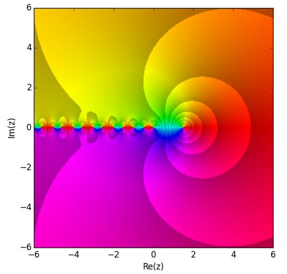
Re ⁡ ψ ( i ) = − γ − ∑ n = 0 ∞ n − 1 n 3 + n 2 + n + 1 , Im ⁡ ψ ( i ) = ∑ n = 0 ∞ 1 n 2 + 1 = 1 2 + π 2 coth ⁡ π .

Roots of the digamma function

The roots of the digamma function are the saddle points of the complex-valued gamma function. Thus they lie all on the real axis. The only one on the positive real axis is the unique minimum of the real-valued gamma function on ℝ⁺ at x₀ = 7000146163214496800♠1.461632144968.... All others occur single between the poles on the negative axis:

x 1 = − 0.504 083 008... , x 2 = − 1.573 498 473... , x 3 = − 2.610 720 868... , x 4 = − 3.635 293 366... , ⋮

Already in 1881, Charles Hermite observed that

x n = − n + 1 ln ⁡ n + o ( 1 ( ln ⁡ n ) 2 )

holds asymptotically. A better approximation of the location of the roots is given by

x n ≈ − n + 1 π arctan ⁡ ( π ln ⁡ n ) n ≥ 2

and using a further term it becomes still better

x n ≈ − n + 1 π arctan ⁡ ( π ln ⁡ n + 1 8 n ) n ≥ 1

which both spring off the reflection formula via

0 = ψ ( 1 − x n ) = ψ ( x n ) + π tan ⁡ π x n

and substituting ψ(x_n) by its not convergent asymptotic expansion. The correct second term of this expansion is 1 / 2n, where the given one works good to approximate roots with small n.

Regarding the zeros, the following infinite sum identities were recently proved by István Mező

∑ n = 0 ∞ 1 x n 2 = γ 2 + π 2 2 , ∑ n = 0 ∞ 1 x n 4 = γ 4 + π 4 9 + 2 3 γ 2 π 2 + 4 γ ζ ( 3 ) .

Here γ is the Euler–Mascheroni constant.

Regularization

The digamma function appears in the regularization of divergent integrals

∫ 0 ∞ d x x + a ,

this integral can be approximated by a divergent general Harmonic series, but the following value can be attached to the series

∑ n = 0 ∞ 1 n + a = − ψ ( a ) .

References

Digamma function Wikipedia

(Text) CC BY-SA

Contents