Semi implicit Euler method

Setting

The semi-implicit Euler method can be applied to a pair of differential equations of the form

where f and g are given functions. Here, x and v may be either scalars or vectors. The equations of motion in Hamiltonian mechanics take this form if the Hamiltonian is of the form

The differential equations are to be solved with the initial condition

The method

The semi-implicit Euler method produces an approximate discrete solution by iterating

where Δt is the time step and t_n = t₀ + nΔt is the time after n steps.

The difference with the standard Euler method is that the semi-implicit Euler method uses v_n+1 in the equation for x_n+1, while the Euler method uses v_n.

Applying the method with negative time step to the computation of ( x n , v n ) from ( x n + 1 , v n + 1 ) and rearranging leads to the second variant of the semi-implicit Euler method

which has similar properties.

The semi-implicit Euler is a first-order integrator, just as the standard Euler method. This means that it commits a global error of the order of Δt. However, the semi-implicit Euler method is a symplectic integrator, unlike the standard method. As a consequence, the semi-implicit Euler method almost conserves the energy (when the Hamiltonian is time-independent). Often, the energy increases steadily when the standard Euler method is applied, making it far less accurate.

Alternating between the two variants of the semi-implicit Euler method leads in one simplification to the Störmer-Verlet integration and in a slightly different simplification to the leapfrog integration, increasing both the order of the error and the order of preservation of energy.

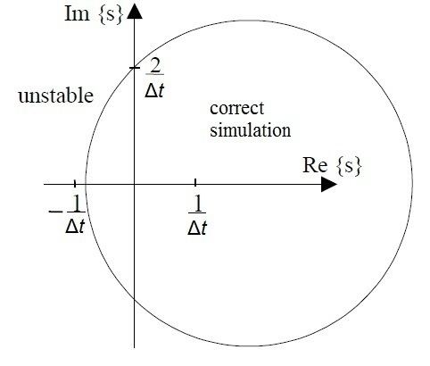
The stability region of the semi-implicit method was presented by Niiranen although the semi-implicit Euler was misleadingly called symmetric Euler in his paper. The semi-implicit method models the simulated system correctly if the complex roots of the characteristic equation are within the circle shown below. For real roots the stability region extends outside the circle for which the criteria is s > − 2 / Δ t

As can be seen, the semi-implicit method can simulate correctly both stable systems that have their roots in the left half plane and unstable systems that have their roots in the right half plane. This is clear advantage over forward (standard) Euler and backward Euler. Forward Euler tends to have less damping than the real system when the negative real parts of the roots get near the imaginary axis and backward Euler may show the system be stable even when the roots are in the right half plane.

Example

The motion of a spring satisfying Hooke's law is given by

The semi-implicit Euler for this equation is

The iteration preserves the modified energy functional E h ( x , v ) = 1 2 ( v 2 + ω 2 x 2 − ω 2 Δ t v x ) exactly, leading to stable periodic orbits (for sufficiently small step size) that deviate by O ( Δ t ) from the exact orbits. The exact circular frequency ω increases in the numerical approximation by a factor of 1 + 1 24 ω 2 Δ t 2 + O ( Δ t 4 ) .