Euler method

Informal geometrical description

Consider the problem of calculating the shape of an unknown curve which starts at a given point and satisfies a given differential equation. Here, a differential equation can be thought of as a formula by which the slope of the tangent line to the curve can be computed at any point on the curve, once the position of that point has been calculated.

The idea is that while the curve is initially unknown, its starting point, which we denote by A 0 , is known (see the picture on top right). Then, from the differential equation, the slope to the curve at A 0 can be computed, and so, the tangent line.

Take a small step along that tangent line up to a point A 1 . Along this small step, the slope does not change too much, so A 1 will be close to the curve. If we pretend that A 1 is still on the curve, the same reasoning as for the point A 0 above can be used. After several steps, a polygonal curve A 0 A 1 A 2 A 3 … is computed. In general, this curve does not diverge too far from the original unknown curve, and the error between the two curves can be made small if the step size is small enough and the interval of computation is finite.

Choose a value h for the size of every step and set t n = t 0 + n h . Now, one step of the Euler method from t n to t n + 1 = t n + h is

The value of y n is an approximation of the solution to the ODE at time t n : y n ≈ y ( t n ) . The Euler method is explicit, i.e. the solution y n + 1 is an explicit function of y i for i ≤ n .

While the Euler method integrates a first-order ODE, any ODE of order N can be represented as a first-order ODE: to treat the equation

we introduce auxiliary variables z 1 ( t ) = y ( t ) , z 2 ( t ) = y ′ ( t ) , … , z N ( t ) = y ( N − 1 ) ( t ) and obtain the equivalent equation

This is a first-order system in the variable z ( t ) and can be handled by Euler's method or, in fact, by any other scheme for first-order systems.

Example

Given the initial value problem

we would like to use the Euler method to approximate y ( 4 ) .

Using step size equal to 1 (h = 1)

The Euler method is

so first we must compute f ( t 0 , y 0 ) . In this simple differential equation, the function f is defined by f ( t , y ) = y . We have

By doing the above step, we have found the slope of the line that is tangent to the solution curve at the point ( 0 , 1 ) . Recall that the slope is defined as the change in y divided by the change in t , or Δ y / Δ t .

The next step is to multiply the above value by the step size h , which we take equal to one here:

Since the step size is the change in t , when we multiply the step size and the slope of the tangent, we get a change in y value. This value is then added to the initial y value to obtain the next value to be used for computations.

The above steps should be repeated to find y 2 , y 3 and y 4 .

Due to the repetitive nature of this algorithm, it can be helpful to organize computations in a chart form, as seen below, to avoid making errors.

The conclusion of this computation is that y 4 = 16 . The exact solution of the differential equation is y ( t ) = e t , so y ( 4 ) = e 4 ≈ 54.598 . Thus, the approximation of the Euler method is not very good in this case. However, as the figure shows, its behaviour is qualitatively right.

Using other step sizes

As suggested in the introduction, the Euler method is more accurate if the step size h is smaller. The table below shows the result with different step sizes. The top row corresponds to the example in the previous section, and the second row is illustrated in the figure.

The error recorded in the last column of the table is the difference between the exact solution at t = 4 and the Euler approximation. In the bottom of the table, the step size is quarter the step size in the previous row, and the error is also approximately half the error in the previous row. This suggests that the error is roughly proportional to the step size, at least for fairly small values of the step size. This is true in general, also for other equations; see the section Global truncation error for more details.

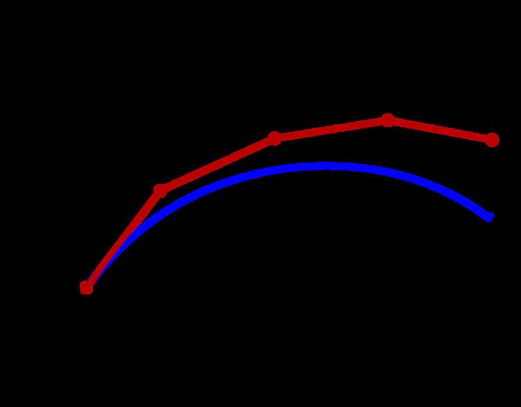
Other methods, such as the midpoint method also illustrated in the figures, behave more favorably: the error of the midpoint method is roughly proportional to the square of the step size. For this reason, the Euler method is said to be a first-order method, while the midpoint method is second order.

We can extrapolate from the above table that the step size needed to get an answer that is correct to three decimal places is approximately 0.00001, meaning that we need 400,000 steps. This large number of steps entails a high computational cost. For this reason, people usually employ alternative, higher-order methods such as Runge–Kutta methods or linear multistep methods, especially if a high accuracy is desired.

Derivation

The Euler method can be derived in a number of ways. Firstly, there is the geometrical description mentioned above.

Another possibility is to consider the Taylor expansion of the function y around t 0 :

The differential equation states that y ′ = f ( t , y ) . If this is substituted in the Taylor expansion and the quadratic and higher-order terms are ignored, the Euler method arises. The Taylor expansion is used below to analyze the error committed by the Euler method, and it can be extended to produce Runge–Kutta methods.

A closely related derivation is to substitute the forward finite difference formula for the derivative,

in the differential equation y ′ = f ( t , y ) . Again, this yields the Euler method. A similar computation leads to the midpoint rule and the backward Euler method.

Finally, one can integrate the differential equation from t 0 to t 0 + h and apply the fundamental theorem of calculus to get:

Now approximate the integral by the left-hand rectangle method (with only one rectangle):

Combining both equations, one finds again the Euler method. This line of thought can be continued to arrive at various linear multistep methods.

Local truncation error

The local truncation error of the Euler method is error made in a single step. It is the difference between the numerical solution after one step, y 1 , and the exact solution at time t 1 = t 0 + h . The numerical solution is given by

For the exact solution, we use the Taylor expansion mentioned in the section Derivation above:

The local truncation error (LTE) introduced by the Euler method is given by the difference between these equations:

This result is valid if y has a bounded third derivative.

This shows that for small h , the local truncation error is approximately proportional to h 2 . This makes the Euler method less accurate (for small h ) than other higher-order techniques such as Runge-Kutta methods and linear multistep methods, for which the local truncation error is proportional to a higher power of the step size.

A slightly different formulation for the local truncation error can be obtained by using the Lagrange form for the remainder term in Taylor's theorem. If y has a continuous second derivative, then there exists a ξ ∈ [ t 0 , t 0 + h ] such that

In the above expressions for the error, the second derivative of the unknown exact solution y can be replaced by an expression involving the right-hand side of the differential equation. Indeed, it follows from the equation y ′ = f ( t , y ) that

Global truncation error

The global truncation error is the error at a fixed time t , after however many steps the methods needs to take to reach that time from the initial time. The global truncation error is the cumulative effect of the local truncation errors committed in each step. The number of steps is easily determined to be ( t − t 0 ) / h , which is proportional to 1 / h , and the error committed in each step is proportional to h 2 (see the previous section). Thus, it is to be expected that the global truncation error will be proportional to h .

This intuitive reasoning can be made precise. If the solution y has a bounded second derivative and f is Lipschitz continuous in its second argument, then the global truncation error (GTE) is bounded by

where M is an upper bound on the second derivative of y on the given interval and L is the Lipschitz constant of f .

The precise form of this bound is of little practical importance, as in most cases the bound vastly overestimates the actual error committed by the Euler method. What is important is that it shows that the global truncation error is (approximately) proportional to h . For this reason, the Euler method is said to be first order.

Numerical stability

The Euler method can also be numerically unstable, especially for stiff equations, meaning that the numerical solution grows very large for equations where the exact solution does not. This can be illustrated using the linear equation

The exact solution is y ( t ) = e − 2.3 t , which decays to zero as t → ∞ . However, if the Euler method is applied to this equation with step size h = 1 , then the numerical solution is qualitatively wrong: it oscillates and grows (see the figure). This is what it means to be unstable. If a smaller step size is used, for instance h = 0.7 , then the numerical solution does decay to zero.

If the Euler method is applied to the linear equation y ′ = k y , then the numerical solution is unstable if the product h k is outside the region

illustrated on the right. This region is called the (linear) instability region. In the example, k equals −2.3, so if h = 1 then h k = − 2.3 which is outside the stability region, and thus the numerical solution is unstable.

This limitation —along with its slow convergence of error with h— means that the Euler method is not often used, except as a simple example of numerical integration.

Rounding errors

The discussion up to now has ignored the consequences of rounding error. In step n of the Euler method, the rounding error is roughly of the magnitude εy_n where ε is the machine epsilon. Assuming that the rounding errors are all of approximately the same size, the combined rounding error in N steps is roughly Nεy₀ if all errors points in the same direction. Since the number of steps is inversely proportional to the step size h, the total rounding error is proportional to ε / h. In reality, however, it is extremely unlikely that all rounding errors point in the same direction. If instead it is assumed that the rounding errors are independent rounding variables, then the total rounding error is proportional to ε / h .

Thus, for extremely small values of the step size, the truncation error will be small but the effect of rounding error may be big. Most of the effect of rounding error can be easily avoided if compensated summation is used in the formula for the Euler method.

Modifications and extensions

A simple modification of the Euler method which eliminates the stability problems noted in the previous section is the backward Euler method:

This differs from the (standard, or forward) Euler method in that the function f is evaluated at the end point of the step, instead of the starting point. The backward Euler method is an implicit method, meaning that the formula for the backward Euler method has y n + 1 on both sides, so when applying the backward Euler method we have to solve an equation. This makes the implementation more costly.

Other modifications of the Euler method that help with stability yield the exponential Euler method or the semi-implicit Euler method.

More complicated methods can achieve a higher order (and more accuracy). One possibility is to use more function evaluations. This is illustrated by the midpoint method which is already mentioned in this article:

This leads to the family of Runge–Kutta methods.

The other possibility is to use more past values, as illustrated by the two-step Adams–Bashforth method:

This leads to the family of linear multistep methods.

In popular culture

In the film Hidden Figures, Katherine Johnson resorts to Euler's method in figuring out how to get astronaut John Glenn back down from orbit.