
 | ||
Similar Discrete mathematics, Mathematical analysis, Calculus | ||
Numerical analysis is the study of algorithms that use numerical approximation (as opposed to general symbolic manipulations) for the problems of mathematical analysis (as distinguished from discrete mathematics).
Contents
- General introduction
- History
- Direct and iterative methods
- Discretization
- Generation and propagation of errors
- Round off
- Truncation and discretization error
- Numerical stability and well posed problems
- Areas of study
- Computing values of functions
- Interpolation extrapolation and regression
- Solving equations and systems of equations
- Solving eigenvalue or singular value problems
- Optimization
- Evaluating integrals
- Differential equations
- Software
- References
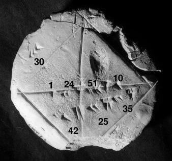
One of the earliest mathematical writings is a Babylonian tablet from the Yale Babylonian Collection (YBC 7289), which gives a sexagesimal numerical approximation of the square root of 2, the length of the diagonal in a unit square. Being able to compute the sides of a triangle (and hence, being able to compute square roots) is extremely important, for instance, in astronomy, carpentry and construction.
Numerical analysis continues this long tradition of practical mathematical calculations. Much like the Babylonian approximation of the square root of 2, modern numerical analysis does not seek exact answers, because exact answers are often impossible to obtain in practice. Instead, much of numerical analysis is concerned with obtaining approximate solutions while maintaining reasonable bounds on errors.
Numerical analysis naturally finds applications in all fields of engineering and the physical sciences, but in the 21st century also the life sciences and even the arts have adopted elements of scientific computations. ordinary differential equations appear in celestial mechanics (planets, stars and galaxies); numerical linear algebra is important for data analysis; stochastic differential equations and Markov chains are essential in simulating living cells for medicine and biology.
Before the advent of modern computers numerical methods often depended on hand interpolation in large printed tables. Since the mid 20th century, computers calculate the required functions instead. These same Interpolation formulas nevertheless continue to be used as part of the software algorithms for solving differential equations.
General introduction
The overall goal of the field of numerical analysis is the design and analysis of techniques to give approximate but accurate solutions to hard problems, the variety of which is suggested by the following:
The rest of this section outlines several important themes of numerical analysis.
History
The field of numerical analysis predates the invention of modern computers by many centuries. Linear interpolation was already in use more than 2000 years ago. Many great mathematicians of the past were preoccupied by numerical analysis, as is obvious from the names of important algorithms like Newton's method, Lagrange interpolation polynomial, Gaussian elimination, or Euler's method.
To facilitate computations by hand, large books were produced with formulas and tables of data such as interpolation points and function coefficients. Using these tables, often calculated out to 16 decimal places or more for some functions, one could look up values to plug into the formulas given and achieve very good numerical estimates of some functions. The canonical work in the field is the NIST publication edited by Abramowitz and Stegun, a 1000-plus page book of a very large number of commonly used formulas and functions and their values at many points. The function values are no longer very useful when a computer is available, but the large listing of formulas can still be very handy.
The mechanical calculator was also developed as a tool for hand computation. These calculators evolved into electronic computers in the 1940s, and it was then found that these computers were also useful for administrative purposes. But the invention of the computer also influenced the field of numerical analysis, since now longer and more complicated calculations could be done.
Direct and iterative methods
Direct methods compute the solution to a problem in a finite number of steps. These methods would give the precise answer if they were performed in infinite precision arithmetic. Examples include Gaussian elimination, the QR factorization method for solving systems of linear equations, and the simplex method of linear programming. In practice, finite precision is used and the result is an approximation of the true solution (assuming stability).
In contrast to direct methods, iterative methods are not expected to terminate in a finite number of steps. Starting from an initial guess, iterative methods form successive approximations that converge to the exact solution only in the limit. A convergence test, often involving the residual, is specified in order to decide when a sufficiently accurate solution has (hopefully) been found. Even using infinite precision arithmetic these methods would not reach the solution within a finite number of steps (in general). Examples include Newton's method, the bisection method, and Jacobi iteration. In computational matrix algebra, iterative methods are generally needed for large problems.
Iterative methods are more common than direct methods in numerical analysis. Some methods are direct in principle but are usually used as though they were not, e.g. GMRES and the conjugate gradient method. For these methods the number of steps needed to obtain the exact solution is so large that an approximation is accepted in the same manner as for an iterative method.
Discretization
Furthermore, continuous problems must sometimes be replaced by a discrete problem whose solution is known to approximate that of the continuous problem; this process is called discretization. For example, the solution of a differential equation is a function. This function must be represented by a finite amount of data, for instance by its value at a finite number of points at its domain, even though this domain is a continuum.
Generation and propagation of errors
The study of errors forms an important part of numerical analysis. There are several ways in which error can be introduced in the solution of the problem.
Round-off
Round-off errors arise because it is impossible to represent all real numbers exactly on a machine with finite memory (which is what all practical digital computers are).
Truncation and discretization error
Truncation errors are committed when an iterative method is terminated or a mathematical procedure is approximated, and the approximate solution differs from the exact solution. Similarly, discretization induces a discretization error because the solution of the discrete problem does not coincide with the solution of the continuous problem. For instance, in the iteration in the sidebar to compute the solution of
Once an error is generated, it will generally propagate through the calculation. For instance, we have already noted that the operation + on a calculator (or a computer) is inexact. It follows that a calculation of the type
What does it mean when we say that the truncation error is created when we approximate a mathematical procedure? We know that to integrate a function exactly requires one to find the sum of infinite trapezoids. But numerically one can find the sum of only finite trapezoids, and hence the approximation of the mathematical procedure. Similarly, to differentiate a function, the differential element approaches zero but numerically we can only choose a finite value of the differential element.
Numerical stability and well-posed problems
Numerical stability is an important notion in numerical analysis. An algorithm is called numerically stable if an error, whatever its cause, does not grow to be much larger during the calculation. This happens if the problem is well-conditioned, meaning that the solution changes by only a small amount if the problem data are changed by a small amount. To the contrary, if a problem is ill-conditioned, then any small error in the data will grow to be a large error.
Both the original problem and the algorithm used to solve that problem can be well-conditioned and/or ill-conditioned, and any combination is possible.
So an algorithm that solves a well-conditioned problem may be either numerically stable or numerically unstable. An art of numerical analysis is to find a stable algorithm for solving a well-posed mathematical problem. For instance, computing the square root of 2 (which is roughly 1.41421) is a well-posed problem. Many algorithms solve this problem by starting with an initial approximation x0 to
Observe that the Babylonian method converges quickly regardless of the initial guess, whereas Method X converges extremely slowly with initial guess x0 = 1.4 and diverges for initial guess x0 = 1.42. Hence, the Babylonian method is numerically stable, while Method X is numerically unstable.
Numerical stability is affected by the number of the significant digits the machine keeps on, if we use a machine that keeps only the four most significant decimal digits, a good example on loss of significance is given by these two equivalent functionsAreas of study
The field of numerical analysis includes many sub-disciplines. Some of the major ones are:
Computing values of functions
One of the simplest problems is the evaluation of a function at a given point. The most straightforward approach, of just plugging in the number in the formula is sometimes not very efficient. For polynomials, a better approach is using the Horner scheme, since it reduces the necessary number of multiplications and additions. Generally, it is important to estimate and control round-off errors arising from the use of floating point arithmetic.
Interpolation, extrapolation, and regression
Interpolation solves the following problem: given the value of some unknown function at a number of points, what value does that function have at some other point between the given points?
Extrapolation is very similar to interpolation, except that now we want to find the value of the unknown function at a point which is outside the given points.
Regression is also similar, but it takes into account that the data is imprecise. Given some points, and a measurement of the value of some function at these points (with an error), we want to determine the unknown function. The least squares-method is one popular way to achieve this.
Solving equations and systems of equations
Another fundamental problem is computing the solution of some given equation. Two cases are commonly distinguished, depending on whether the equation is linear or not. For instance, the equation
Much effort has been put in the development of methods for solving systems of linear equations. Standard direct methods, i.e., methods that use some matrix decomposition are Gaussian elimination, LU decomposition, Cholesky decomposition for symmetric (or hermitian) and positive-definite matrix, and QR decomposition for non-square matrices. Iterative methods such as the Jacobi method, Gauss–Seidel method, successive over-relaxation and conjugate gradient method are usually preferred for large systems. General iterative methods can be developed using a matrix splitting.
Root-finding algorithms are used to solve nonlinear equations (they are so named since a root of a function is an argument for which the function yields zero). If the function is differentiable and the derivative is known, then Newton's method is a popular choice. Linearization is another technique for solving nonlinear equations.
Solving eigenvalue or singular value problems
Several important problems can be phrased in terms of eigenvalue decompositions or singular value decompositions. For instance, the spectral image compression algorithm is based on the singular value decomposition. The corresponding tool in statistics is called principal component analysis.
Optimization
Optimization problems ask for the point at which a given function is maximized (or minimized). Often, the point also has to satisfy some constraints.
The field of optimization is further split in several subfields, depending on the form of the objective function and the constraint. For instance, linear programming deals with the case that both the objective function and the constraints are linear. A famous method in linear programming is the simplex method.
The method of Lagrange multipliers can be used to reduce optimization problems with constraints to unconstrained optimization problems.
Evaluating integrals
Numerical integration, in some instances also known as numerical quadrature, asks for the value of a definite integral. Popular methods use one of the Newton–Cotes formulas (like the midpoint rule or Simpson's rule) or Gaussian quadrature. These methods rely on a "divide and conquer" strategy, whereby an integral on a relatively large set is broken down into integrals on smaller sets. In higher dimensions, where these methods become prohibitively expensive in terms of computational effort, one may use Monte Carlo or quasi-Monte Carlo methods (see Monte Carlo integration), or, in modestly large dimensions, the method of sparse grids.
Differential equations
Numerical analysis is also concerned with computing (in an approximate way) the solution of differential equations, both ordinary differential equations and partial differential equations.
Partial differential equations are solved by first discretizing the equation, bringing it into a finite-dimensional subspace. This can be done by a finite element method, a finite difference method, or (particularly in engineering) a finite volume method. The theoretical justification of these methods often involves theorems from functional analysis. This reduces the problem to the solution of an algebraic equation.
Software
Since the late twentieth century, most algorithms are implemented in a variety of programming languages. The Netlib repository contains various collections of software routines for numerical problems, mostly in Fortran and C. Commercial products implementing many different numerical algorithms include the IMSL and NAG libraries; a free alternative is the GNU Scientific Library.
There are several popular numerical computing applications such as MATLAB, TK Solver, S-PLUS, and IDL as well as free and open source alternatives such as FreeMat, Scilab, GNU Octave (similar to Matlab), IT++ (a C++ library), R (similar to S-PLUS) and certain variants of Python. Performance varies widely: while vector and matrix operations are usually fast, scalar loops may vary in speed by more than an order of magnitude.
Many computer algebra systems such as Mathematica also benefit from the availability of arbitrary precision arithmetic which can provide more accurate results.
Also, any spreadsheet software can be used to solve simple problems relating to numerical analysis.