Big O notation

Formal definition

Let f and g be two functions defined on some subset of the real numbers. One writes

f ( x ) = O ( g ( x ) )  as  x → ∞

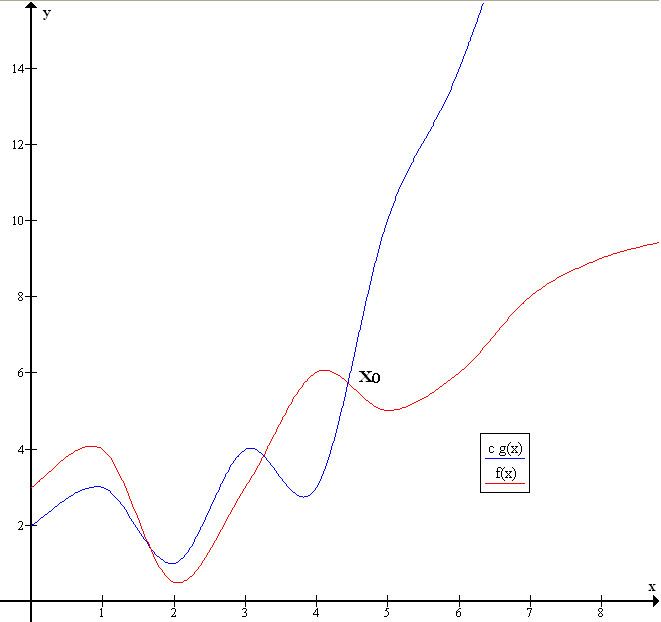
if and only if there is a positive constant M such that for all sufficiently large values of x, the absolute value of f(x) is at most M multiplied by the absolute value of g(x). That is, f(x) = O(g(x)) if and only if there exists a positive real number M and a real number x₀ such that

| f ( x ) | ≤ M | g ( x ) |  for all  x ≥ x 0 .

In many contexts, the assumption that we are interested in the growth rate as the variable x goes to infinity is left unstated, and one writes more simply that

f ( x ) = O ( g ( x ) ) .

The notation can also be used to describe the behavior of f near some real number a (often, a = 0): we say

f ( x ) = O ( g ( x ) )  as  x → a

if and only if there exist positive numbers δ and M such that

| f ( x ) | ≤ M | g ( x ) |  when  0 < | x − a | < δ .

If g(x) is non-zero for values of x sufficiently close to a, both of these definitions can be unified using the limit superior:

f ( x ) = O ( g ( x ) )  as  x → a

if and only if

lim sup x → a | f ( x ) g ( x ) | < ∞ .

Example

In typical usage, the formal definition of O notation is not used directly; rather, the O notation for a function f is derived by the following simplification rules:

If f(x) is a sum of several terms, if there is one with largest growth rate, it can be kept, and all others omitted.

If f(x) is a product of several factors, any constants (terms in the product that do not depend on x) can be omitted.

For example, let f(x) = 6x⁴ − 2x³ + 5, and suppose we wish to simplify this function, using O notation, to describe its growth rate as x approaches infinity. This function is the sum of three terms: 6x⁴, −2x³, and 5. Of these three terms, the one with the highest growth rate is the one with the largest exponent as a function of x, namely 6x⁴. Now one may apply the second rule: 6x⁴ is a product of 6 and x⁴ in which the first factor does not depend on x. Omitting this factor results in the simplified form x⁴. Thus, we say that f(x) is a "big-oh" of (x⁴). Mathematically, we can write f(x) = O(x⁴). One may confirm this calculation using the formal definition: let f(x) = 6x⁴ − 2x³ + 5 and g(x) = x⁴. Applying the formal definition from above, the statement that f(x) = O(x⁴) is equivalent to its expansion,

| f ( x ) | ≤ M | x 4 |

for some suitable choice of x₀ and M and for all x > x₀. To prove this, let x₀ = 1 and M = 13. Then, for all x > x₀:

| 6 x 4 − 2 x 3 + 5 | ≤ 6 x 4 + | 2 x 3 | + 5 ≤ 6 x 4 + 2 x 4 + 5 x 4 = 13 x 4

so

| 6 x 4 − 2 x 3 + 5 | ≤ 13 x 4 .

Usage

Big O notation has two main areas of application. In mathematics, it is commonly used to describe how closely a finite series approximates a given function, especially in the case of a truncated Taylor series or asymptotic expansion. In computer science, it is useful in the analysis of algorithms. In both applications, the function g(x) appearing within the O(...) is typically chosen to be as simple as possible, omitting constant factors and lower order terms. There are two formally close, but noticeably different, usages of this notation: infinite asymptotics and infinitesimal asymptotics. This distinction is only in application and not in principle, however—the formal definition for the "big O" is the same for both cases, only with different limits for the function argument.

Infinite asymptotics

Big O notation is useful when analyzing algorithms for efficiency. For example, the time (or the number of steps) it takes to complete a problem of size n might be found to be T(n) = 4n² − 2n + 2. As n grows large, the n² term will come to dominate, so that all other terms can be neglected—for instance when n = 500, the term 4n² is 1000 times as large as the 2n term. Ignoring the latter would have negligible effect on the expression's value for most purposes. Further, the coefficients become irrelevant if we compare to any other order of expression, such as an expression containing a term n³ or n⁴. Even if T(n) = 1,000,000n², if U(n) = n³, the latter will always exceed the former once n grows larger than 1,000,000 (T(1,000,000) = 1,000,000³= U(1,000,000)). Additionally, the number of steps depends on the details of the machine model on which the algorithm runs, but different types of machines typically vary by only a constant factor in the number of steps needed to execute an algorithm. So the big O notation captures what remains: we write either

  T ( n ) = O ( n 2 )

or

T ( n ) ∈ O ( n 2 )

and say that the algorithm has order of n² time complexity. Note that "=" is not meant to express "is equal to" in its normal mathematical sense, but rather a more colloquial "is", so the second expression is sometimes considered more accurate (see the "Equals sign" discussion below) while the first is considered by some as an Abuse of notation.

Infinitesimal asymptotics

Big O can also be used to describe the error term in an approximation to a mathematical function. The most significant terms are written explicitly, and then the least-significant terms are summarized in a single big O term. Consider, for example, the exponential series and two expressions of it that are valid when x is small:

e x = 1 + x + x 2 2 ! + x 3 3 ! + x 4 4 ! + ⋯ for all  x = 1 + x + x 2 2 + O ( x 3 ) as  x → 0 = 1 + x + O ( x 2 ) as  x → 0

The second expression (the one with O(x³)) means the absolute-value of the error e^x − (1 + x + x²/2) is at most some constant times |x³| when x is close enough to 0.

Properties

If the function f can be written as a finite sum of other functions, then the fastest growing one determines the order of f(n). For example,

f ( n ) = 9 log ⁡ n + 5 ( log ⁡ n ) 3 + 3 n 2 + 2 n 3 = O ( n 3 ) , as  n → ∞ .

In particular, if a function may be bounded by a polynomial in n, then as n tends to infinity, one may disregard lower-order terms of the polynomial. Another thing to notice is the sets O(n^c) and O(cⁿ) are very different. If c is greater than one, then the latter grows much faster. A function that grows faster than n^c for any c is called superpolynomial. One that grows more slowly than any exponential function of the form cⁿ is called subexponential. An algorithm can require time that is both superpolynomial and subexponential; examples of this include the fastest known algorithms for integer factorization and the function n^{log n}.

We may ignore any powers of n inside of the logarithms. The set O(log n) is exactly the same as O(log(n^c)). The logarithms differ only by a constant factor (since log(n^c) = c log n) and thus the big O notation ignores that. Similarly, logs with different constant bases are equivalent. On the other hand, exponentials with different bases are not of the same order. For example, 2ⁿ and 3ⁿ are not of the same order.

Changing units may or may not affect the order of the resulting algorithm. Changing units is equivalent to multiplying the appropriate variable by a constant wherever it appears. For example, if an algorithm runs in the order of n², replacing n by cn means the algorithm runs in the order of c²n², and the big O notation ignores the constant c². This can be written as c²n² = O(n²). If, however, an algorithm runs in the order of 2ⁿ, replacing n with cn gives 2^cn = (2^c)ⁿ. This is not equivalent to 2ⁿ in general. Changing variables may also affect the order of the resulting algorithm. For example, if an algorithm's run time is O(n) when measured in terms of the number n of digits of an input number x, then its run time is O(log x) when measured as a function of the input number x itself, because n = O(log x).

Product

f 1 = O ( g 1 )  and  f 2 = O ( g 2 ) ⇒ f 1 f 2 = O ( g 1 g 2 ) f ⋅ O ( g ) = O ( f g )

Sum

f 1 = O ( g 1 )  and  f 2 = O ( g 2 ) ⇒ f 1 + f 2 = O ( | g 1 | + | g 2 | )

This implies f 1 = O ( g )  and  f 2 = O ( g ) ⇒ f 1 + f 2 ∈ O ( g ) , which means that O ( g ) is a convex cone.

If f and g are positive functions, f + O ( g ) = O ( f + g )

Multiplication by a constant

Let k be a constant. Then:   O ( k g ) = O ( g ) if k is nonzero. f = O ( g ) ⇒ k f = O ( g ) .

Multiple variables

Big O (and little o, and Ω...) can also be used with multiple variables. To define Big O formally for multiple variables, suppose f and g are two functions defined on some subset of R n . We say

f ( x → )  is  O ( g ( x → ) )  as  x → → ∞

if and only if

∃ M ∃ C > 0  such that for all  x →  with  x i ≥ M  for some  i , | f ( x → ) | ≤ C | g ( x → ) | .

Equivalently, the condition that x i ≥ M for some i can be replaced with the condition that ∥ x → ∥ ∞ ≥ M , where ∥ x → ∥ ∞ denotes the Chebyshev norm. For example, the statement

f ( n , m ) = n 2 + m 3 + O ( n + m )  as  n , m → ∞

asserts that there exist constants C and M such that

∀ ∥ ( n , m ) ∥ ∞ ≥ M : | g ( n , m ) | ≤ C | n + m | ,

where g(n,m) is defined by

f ( n , m ) = n 2 + m 3 + g ( n , m ) .

Note that this definition allows all of the coordinates of x → to increase to infinity. In particular, the statement

f ( n , m ) = O ( n m )  as  n , m → ∞

(i.e., ∃ C ∃ M ∀ n ∀ m … ) is quite different from

∀ m : f ( n , m ) = O ( n m )  as  n → ∞

(i.e., ∀ m ∃ C ∃ M ∀ n … ).

This is not the only generalization of big O to multivariate functions, and in practice, there is some inconsistency in the choice of definition.

Equals sign

The statement "f(x) is O(g(x))" as defined above is usually written as f(x) = O(g(x)). Some consider this to be an abuse of notation, since the use of the equals sign could be misleading as it suggests a symmetry that this statement does not have. As de Bruijn says, O(x) = O(x²) is true but O(x²) = O(x) is not. Knuth describes such statements as "one-way equalities", since if the sides could be reversed, "we could deduce ridiculous things like n = n² from the identities n = O(n²) and n² = O(n²)."

For these reasons, it would be more precise to use set notation and write f(x) ∈ O(g(x)), thinking of O(g(x)) as the class of all functions h(x) such that |h(x)| ≤ C|g(x)| for some constant C. However, the use of the equals sign is customary. Knuth pointed out that "mathematicians customarily use the = sign as they use the word 'is' in English: Aristotle is a man, but a man isn't necessarily Aristotle."

Other arithmetic operators

Big O notation can also be used in conjunction with other arithmetic operators in more complicated equations. For example, h(x) + O(f(x)) denotes the collection of functions having the growth of h(x) plus a part whose growth is limited to that of f(x). Thus,

g ( x ) = h ( x ) + O ( f ( x ) )

expresses the same as

g ( x ) − h ( x ) = O ( f ( x ) ) .

Example

Suppose an algorithm is being developed to operate on a set of n elements. Its developers are interested in finding a function T(n) that will express how long the algorithm will take to run (in some arbitrary measurement of time) in terms of the number of elements in the input set. The algorithm works by first calling a subroutine to sort the elements in the set and then perform its own operations. The sort has a known time complexity of O(n²), and after the subroutine runs the algorithm must take an additional 55n³ + 2n + 10 steps before it terminates. Thus the overall time complexity of the algorithm can be expressed as T(n) = 55n³ + O(n²). Here the terms 2n+10 are subsumed within the faster-growing O(n²). Again, this usage disregards some of the formal meaning of the "=" symbol, but it does allow one to use the big O notation as a kind of convenient placeholder.

Declaration of variables

Another feature of the notation, although less exceptional, is that function arguments may need to be inferred from the context when several variables are involved. The following two right-hand side big O notations have dramatically different meanings:

f ( m ) = O ( m n ) , g ( n ) = O ( m n ) .

The first case states that f(m) exhibits polynomial growth, while the second, assuming m > 1, states that g(n) exhibits exponential growth. To avoid confusion, some authors use the notation

g ( x ) = O ( f ( x ) ) .

rather than the less explicit

g = O ( f ) ,

Multiple usages

In more complicated usage, O(...) can appear in different places in an equation, even several times on each side. For example, the following are true for n → ∞

( n + 1 ) 2 = n 2 + O ( n )   ( n + O ( n 1 / 2 ) ) ( n + O ( log ⁡ n ) ) 2 = n 3 + O ( n 5 / 2 )   n O ( 1 ) = O ( e n ) .  

The meaning of such statements is as follows: for any functions which satisfy each O(...) on the left side, there are some functions satisfying each O(...) on the right side, such that substituting all these functions into the equation makes the two sides equal. For example, the third equation above means: "For any function f(n) = O(1), there is some function g(n) =O(eⁿ) such that n^f(n) = g(n)." In terms of the "set notation" above, the meaning is that the class of functions represented by the left side is a subset of the class of functions represented by the right side. In this use the "=" is a formal symbol that unlike the usual use of "=" is not a symmetric relation. Thus for example n^O(1) = O(eⁿ) does not imply the false statement O(eⁿ) = n^O(1)

Orders of common functions

Here is a list of classes of functions that are commonly encountered when analyzing the running time of an algorithm. In each case, c is a positive constant and n increases without bound. The slower-growing functions are generally listed first.

The statement f ( n ) = O ( n ! ) is sometimes weakened to f ( n ) = O ( n n ) to derive simpler formulas for asymptotic complexity. For any k > 0 and c > 0 , O ( n c ( log ⁡ n ) k ) is a subset of O ( n c + ε ) for any ε > 0 , so may be considered as a polynomial with some bigger order.

Related asymptotic notations

Big O is the most commonly used asymptotic notation for comparing functions, although in many cases Big O may be replaced with Big Theta Θ for asymptotically tighter bounds. Here, we define some related notations in terms of Big O, progressing up to the family of Bachmann–Landau notations to which Big O notation belongs.

Little-o notation

The informal assertion "f(x) is little-o of g(x)" is formally written

f(x) = o(g(x)) ,

or in set notation f(x) ∈ o(g(x)). Intuitively, it means that g(x) grows much faster than f(x), or similarly, that the growth of f(x) is nothing compared to that of g(x).

It assumes that f and g are both functions of one variable. Formally, f(n) = o(g(n)) (or f(n) ∈ o(g(n))) as n → ∞ means that for every positive constant ε there exists a constant N such that

| f ( n ) | ≤ ε | g ( n ) | for all  n ≥ N   .

Note the difference between the earlier formal definition for the big-O notation, and the present definition of little-o: while the former has to be true for at least one constant M the latter must hold for every positive constant ε, however small. In this way, little-o notation makes a stronger statement than the corresponding big-O notation: every function that is little-o of g is also big-O of g, but not every function that is big-O of g is also little-o of g (for instance g itself is not, unless it is identically zero near ∞).

If g(x) is nonzero, or at least becomes nonzero beyond a certain point, the relation f(x) = o(g(x)) is equivalent to

lim x → ∞ f ( x ) g ( x ) = 0.

For example,

2 x = o ( x 2 )

2 x 2 ≠ o ( x 2 )

1 / x = o ( 1 )

Little-o notation is common in mathematics but rarer in computer science. In computer science, the variable (and function value) is most often a natural number. In mathematics, the variable and function values are often real numbers. The following properties (expressed in the more recent, set-theoretical notation) can be useful:

c ⋅ o ( f ) = o ( f ) for c ≠ 0

o ( f ) o ( g ) ⊆ o ( f g )

o ( o ( f ) ) ⊆ o ( f )

o ( f ) ⊂ O ( f ) (and thus the above properties apply with most combinations of o and O).

As with big O notation, the statement "f(x) is o(g(x)) " is usually written as f(x) = o(g(x)), which some consider an abuse of notation.

Big Omega notation

There are two very widespread and incompatible definitions of the statement

f ( x ) = Ω ( g ( x ) )   ( x → a ) ,

where a is some real number, ∞, or −∞, where f and g are real functions defined in a neighbourhood of a, and where g is positive in this neighbourhood.

The first one (chronologically) is used in analytic number theory, and the other one in computational complexity theory. When the two subjects meet, this situation is bound to generate confusion.

The Hardy–Littlewood definition

In 1914 G.H. Hardy and J.E. Littlewood introduced the new symbol Ω , which is defined as follows:

f ( x ) = Ω ( g ( x ) )   ( x → ∞ ) ⇔ lim sup x → ∞ | f ( x ) g ( x ) | > 0 .

Thus f ( x ) = Ω ( g ( x ) ) is the negation of f ( x ) = o ( g ( x ) ) .

In 1916 the same authors introduced the two new symbols Ω R and Ω L , thus defined:

f ( x ) = Ω R ( g ( x ) )   ( x → ∞ ) ⇔ lim sup x → ∞ f ( x ) g ( x ) > 0 ; f ( x ) = Ω L ( g ( x ) )   ( x → ∞ ) ⇔ lim inf x → ∞ f ( x ) g ( x ) < 0 .

Hence f ( x ) = Ω R ( g ( x ) ) is the negation of f ( x ) < o ( g ( x ) ) , and f ( x ) = Ω L ( g ( x ) ) is the negation of f ( x ) > o ( g ( x ) ) .

Contrary to a later assertion of D.E. Knuth, Edmund Landau did use these three symbols, with the same meanings, in 1924.

These Hardy-Littlewood symbols are prototypes, which after Landau were never used again exactly thus.

Ω R became Ω + , and Ω L became Ω − .

These three symbols Ω , Ω + , Ω − , as well as f ( x ) = Ω ± ( g ( x ) ) (meaning that f ( x ) = Ω + ( g ( x ) ) and f ( x ) = Ω − ( g ( x ) ) are both satisfied), are now currently used in analytic number theory.

Simple examples

We have

sin ⁡ x = Ω ( 1 )   ( x → ∞ ) ,

and more precisely

sin ⁡ x = Ω ± ( 1 )   ( x → ∞ ) .

We have

sin ⁡ x + 1 = Ω ( 1 )   ( x → ∞ ) ,

and more precisely

sin ⁡ x + 1 = Ω + ( 1 )   ( x → ∞ ) ;

however

sin ⁡ x + 1 ≠ Ω − ( 1 )   ( x → ∞ ) .

The Knuth definition

In 1976 Donald Knuth published a paper to justify his use of the Ω -symbol to describe a stronger property. Knuth wrote: "For all the applications I have seen so far in computer science, a stronger requirement […] is much more appropriate". He defined

f ( x ) = Ω ( g ( x ) ) ⇔ g ( x ) = O ( f ( x ) )

with the comment: "Although I have changed Hardy and Littlewood's definition of Ω , I feel justified in doing so because their definition is by no means in wide use, and because there are other ways to say what they want to say in the comparatively rare cases when their definition applies". However, the Hardy–Littlewood definition had been used for at least 25 years.

Family of Bachmann–Landau notations

Aside from the big O notation, the Big Theta Θ and big Omega Ω notations are the two most often used in computer science.

Aside from the big O notation, the small o, big Omega Ω and ∼ notations are the three most often used in number theory; the small omega ω notation is never used in number theory.

Use in computer science

Informally, especially in computer science, the Big O notation often is permitted to be somewhat abused to describe an asymptotic tight bound where using Big Theta Θ notation might be more factually appropriate in a given context. For example, when considering a function T(n) = 73n³ + 22n² + 58, all of the following are generally acceptable, but tighter bounds (i.e., numbers 2 and 3 below) are usually strongly preferred over looser bounds (i.e., number 1 below).

1. T(n) = O(n¹⁰⁰)
2. T(n) = O(n³)
3. T(n) = Θ(n³)

The equivalent English statements are respectively:

1. T(n) grows asymptotically no faster than n¹⁰⁰
2. T(n) grows asymptotically no faster than n³
3. T(n) grows asymptotically as fast as n³.

So while all three statements are true, progressively more information is contained in each. In some fields, however, the big O notation (number 2 in the lists above) would be used more commonly than the Big Theta notation (bullets number 3 in the lists above). For example, if T(n) represents the running time of a newly developed algorithm for input size n, the inventors and users of the algorithm might be more inclined to put an upper asymptotic bound on how long it will take to run without making an explicit statement about the lower asymptotic bound.

Other notation

In Introduction to Algorithms, Cormen, Leiserson, Rivest and Stein consider the set of functions g to which some function f belongs when it satisfies

f ( n ) = O ( g ( n ) )   ( n → ∞ ) .

In a correct notation this set can for instance be called O(g), where

O ( g ) = { f : there exist positive constants c and n 0 such that 0 ≤ f ( n ) ≤ c g ( n ) for all n ≥ n 0 } .

The authors state that the use of equality operator (=) to denote set membership rather than the set membership operator (∈) is an abuse of notation, but that doing so has advantages. Inside an equation or inequality, the use of asymptotic notation stands for an anonymous function in the set O(g), which eliminates lower-order terms, and helps to reduce inessential clutter in equations, for example:

2 n 2 + 3 n + 1 = 2 n 2 + O ( n ) .

Extensions to the Bachmann–Landau notations

Another notation sometimes used in computer science is Õ (read soft-O): f(n) = Õ(g(n)) is shorthand for f(n) = O(g(n) log^k g(n)) for some k. Essentially, it is big O notation, ignoring logarithmic factors because the growth-rate effects of some other super-logarithmic function indicate a growth-rate explosion for large-sized input parameters that is more important to predicting bad run-time performance than the finer-point effects contributed by the logarithmic-growth factor(s). This notation is often used to obviate the "nitpicking" within growth-rates that are stated as too tightly bounded for the matters at hand (since log^k n is always o(n^ε) for any constant k and any ε > 0).

Also the L notation, defined as

L n [ α , c ] = e ( c + o ( 1 ) ) ( ln ⁡ n ) α ( ln ⁡ ln ⁡ n ) 1 − α

is convenient for functions that are between polynomial and exponential in terms of ln ⁡ n .

Generalizations and related usages

The generalization to functions taking values in any normed vector space is straightforward (replacing absolute values by norms), where f and g need not take their values in the same space. A generalization to functions g taking values in any topological group is also possible. The "limiting process" x→x_o can also be generalized by introducing an arbitrary filter base, i.e. to directed nets f and g. The o notation can be used to define derivatives and differentiability in quite general spaces, and also (asymptotical) equivalence of functions,

f ∼ g ⟺ ( f − g ) ∈ o ( g )

which is an equivalence relation and a more restrictive notion than the relationship "f is Θ(g)" from above. (It reduces to lim f / g = 1 if f and g are positive real valued functions.) For example, 2x is Θ(x), but 2x − x is not o(x).

History (Bachmann–Landau, Hardy, and Vinogradov notations)

The symbol O was first introduced by number theorist Paul Bachmann in 1894, in the second volume of his book Analytische Zahlentheorie ("analytic number theory"), the first volume of which (not yet containing big O notation) was published in 1892. The number theorist Edmund Landau adopted it, and was thus inspired to introduce in 1909 the notation o; hence both are now called Landau symbols. These notations were used in applied mathematics during the 1950s for asymptotic analysis. The big O was popularized in computer science by Donald Knuth, who re-introduced the related Omega and Theta notations. Knuth also noted that the Omega notation had been introduced by Hardy and Littlewood under a different meaning "≠o" (i.e. "is not an o of"), and proposed the above definition. Hardy and Littlewood's original definition (which was also used in one paper by Landau) is still used in number theory (where Knuth's definition is never used). In fact, Landau also used in 1924, in the paper just mentioned, the symbols Ω R ("right") and Ω L ("left"), which were introduced in 1918 by Hardy and Littlewood, and which were precursors for the modern symbols Ω + ("is not smaller than a small o of") and Ω − ("is not larger than a small o of"). Thus the Omega symbols (with their original meanings) are sometimes also referred to as "Landau symbols".

Also, Landau never used the Big Theta and small omega symbols.

Hardy's symbols were (in terms of the modern O notation)

f ≼ g ⟺ f ∈ O ( g )   and   f ≺ g ⟺ f ∈ o ( g ) ;

(Hardy however never defined or used the notation ≺ ≺ , nor ≪ , as it has been sometimes reported). It should also be noted that Hardy introduces the symbols ≼ and ≺ (as well as some other symbols) in his 1910 tract "Orders of Infinity", and makes use of it only in three papers (1910–1913). In his nearly 400 remaining papers and books he consistently uses the Landau symbols O and o.

Hardy's notation is not used anymore. On the other hand, in the 1930s, the Russian number theorist Ivan Matveyevich Vinogradov introduced his notation ≪ , which has been increasingly used in number theory instead of the O notation. We have

f ≪ g ⟺ f ∈ O ( g ) ,

and frequently both notations are used in the same paper.

The big-O originally stands for "order of" ("Ordnung", Bachmann 1894), and is thus a Latin letter. Neither Bachmann nor Landau ever call it "Omicron". The symbol was much later on (1976) viewed by Knuth as a capital omicron, probably in reference to his definition of the symbol Omega. The digit zero should not be used.