In numerical analysis, fixed-point iteration is a method of computing fixed points of iterated functions.
More specifically, given a function f defined on the real numbers with real values and given a point x 0 in the domain of f , the fixed point iteration is
x n + 1 = f ( x n ) , n = 0 , 1 , 2 , … which gives rise to the sequence x 0 , x 1 , x 2 , … which is hoped to converge to a point x . If f is continuous, then one can prove that the obtained x is a fixed point of f , i.e.,
f ( x ) = x . More generally, the function f can be defined on any metric space with values in that same space.
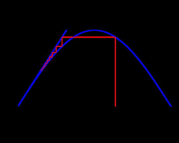
A first simple and useful example is the Babylonian method for computing the square root of a>0, which consists in taking f ( x ) = 1 2 ( a x + x ) , i.e. the mean value of x and a/x, to approach the limit x = a (from whatever starting point x 0 ≫ 0 ). This is a special case of Newton's method quoted below.The fixed-point iteration x n + 1 = cos x n converges to the unique fixed point of the function f ( x ) = cos x for any starting point x 0 . This example does satisfy the assumptions of the Banach fixed point theorem. Hence, the error after n steps satisfies | x n − x 0 | ≤ q n 1 − q | x 1 − x 0 | = C q n (where we can take q = 0.85 , if we start from x 0 = 1 .) When the error is less than a multiple of q n for some constant q, we say that we have linear convergence. The Banach fixed-point theorem allows one to obtain fixed-point iterations with linear convergence.The fixed-point iteration x n + 1 = 2 x n will diverge unless x 0 = 0 . We say that the fixed point of f ( x ) = 2 x is repelling.The requirement that f is continuous is important, as the following example shows. The iteration x n + 1 = { x n 2 , x n ≠ 0 1 , x n = 0 converges to 0 for all values of x 0 . However, 0 is not a fixed point of the function
f ( x ) = { x 2 , x ≠ 0 1 , x = 0 as this function is not continuous at x = 0 , and in fact has no fixed points.
Newton's method for finding roots of a given differentiable function f ( x ) isIf we write
g ( x ) = x − f ( x ) f ′ ( x ) , we may rewrite the Newton iteration as the fixed-point iteration
x n + 1 = g ( x n ) .If this iteration converges to a fixed point
x of
g, then
x = g ( x ) = x − f ( x ) f ′ ( x ) , so
f ( x ) / f ′ ( x ) = 0. The reciprocal of anything is nonzero, therefore
f(x) = 0:
x is a
root of
f. Under the assumptions of the Banach fixed point theorem, the Newton iteration, framed as the fixed point method, demonstrates linear convergence. However, a more detailed analysis shows quadratic convergence, i.e.,
| x n − x | < C q 2 n , under certain circumstances.
Halley's method is similar to Newton's method but, when it works correctly, its error is | x n − x | < C q 3 n (cubic convergence). In general, it is possible to design methods that converge with speed C q k n for any k ∈ N . As a general rule, the higher the k, the less stable it is, and the more computationally expensive it gets. For these reasons, higher order methods are typically not used.Runge–Kutta methods and numerical ordinary differential equation solvers in general can be viewed as fixed point iterations. Indeed, the core idea when analyzing the A-stability of ODE solvers is to start with the special case y ′ = a y , where a is a complex number, and to check whether the ODE solver converges to the fixed point y = 0 whenever the real part of a is negative.The Picard–Lindelöf theorem, which shows that ordinary differential equations have solutions, is essentially an application of the Banach fixed point theorem to a special sequence of functions which forms a fixed point iteration, constructing the solution to the equation. Solving an ODE in this way is called Picard iteration, Picard's method, or the Picard iterative process.The goal seeking function in Excel can be used to find solutions to the Colebrook equation to an accuracy of 15 significant figures.Some of the "successive approximation" schemes used in dynamic programming to solve Bellman's functional equation are based on fixed point iterations in the space of the return function.If a function f defined on the real line with real values is Lipschitz continuous with Lipschitz constant L < 1 , then this function has precisely one fixed point, and the fixed-point iteration converges towards that fixed point for any initial guess x 0 . This theorem can be generalized to any metric space.Proof of this theorem:Since
f is Lipschitz continuous with Lipschitz constant
L < 1 , then for the sequence
{ x n , n = 0 , 1 , 2 , … } , we have:andCombining the above inequalities yields:Since
L < 1 ,
L n − 1 → 0 as
n → ∞ . Therefore, we can show
{ x n } is a Cauchy sequence and thus it converges to a point
x ∗ .For the iteration
x n = f ( x n − 1 ) , let
n go to infinity on both sides of the equation, we obtain
x ∗ = f ( x ∗ ) . This shows that
x ∗ is the fixed point for
f . So we proved the iteration will eventually converge to a fixed-point.This property is very useful because not all iterations can arrive at a convergent fixed-point. When constructing a fixed-point iteration, it is very important to make sure it converges. There are several fixed-point theorems to guarantee the existence of the fixed point, but since the iteration function is continuous, we can usually use the above theorem to test if an iteration converges or not. The proof of the generalized theorem to metric space is similar.
The speed of convergence of the iteration sequence can be increased by using a convergence acceleration method such as Aitken's delta-squared process. The application of Aitken's method to fixed-point iteration is known as Steffensen's method, and it can be shown that Steffensen's method yields a rate of convergence that is at least quadratic.