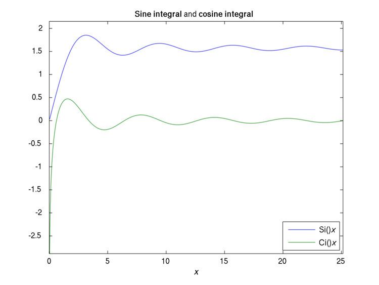
The different sine integral definitions are
Note that the integrand sin x / x is the sinc function, and also the zeroth spherical Bessel function. Since sinc is an even entire function (holomorphic over the entire complex plane), Si is entire, odd, and the integral in its definition can be taken along any path connecting the endpoints.
By definition, Si(x) is the antiderivative of sin x / x which is zero for x = 0, and si(x) is the antiderivative of sin x / x which is zero for x = ∞. Their difference is given by the Dirichlet integral,
In signal processing, the oscillations of the sine integral cause overshoot and ringing artifacts when using the sinc filter, and frequency domain ringing if using a truncated sinc filter as a low-pass filter.
Related is the Gibbs phenomenon: if the sine integral is considered as the convolution of the sinc function with the heaviside step function, this corresponds to truncating the Fourier series, which is the cause of the Gibbs phenomenon.
The different cosine integral definitions are
where γ is the Euler–Mascheroni constant. Some texts use ci instead of Ci.
Ci(x) is the antiderivative of cos x / x (which vanishes at x → ∞ ). The two definitions are related by
Cin is an even entire function.
The hyperbolic sine integral is defined as
It is related to the ordinary sine integral by
The hyperbolic cosine integral is
where γ is the Euler–Mascheroni constant.
It has the series expansion Chi ( x ) = γ + ln ( x ) + 1 4 x 2 + 1 96 x 4 + 1 4320 x 6 + 1 322560 x 8 + 1 36288000 x 10 + O ( x 12 ) .
Trigonometric integrals can be understood in terms of the so-called "auxiliary functions"
f ( x ) ≡ ∫ 0 ∞ sin ( t ) t + x d t = ∫ 0 ∞ e − x t t 2 + 1 d t = Ci ( x ) sin ( x ) + [ π 2 − Si ( x ) ] cos ( x ) g ( x ) ≡ ∫ 0 ∞ cos ( t ) t + x d t = ∫ 0 ∞ t e − x t t 2 + 1 d t = − Ci ( x ) cos ( x ) + [ π 2 − Si ( x ) ] sin ( x ) .
Using these functions, the trigonometric integrals may be re-expressed as (cf Abramowitz & Stegun, p. 232)
Si ( x ) = π 2 − f ( x ) cos ( x ) − g ( x ) sin ( x ) Ci ( x ) = f ( x ) sin ( x ) − g ( x ) cos ( x ) . The spiral formed by parametric plot of si , ci is known as Nielsen's spiral. It is also referred to as the Euler spiral, the Cornu spiral, a clothoid, or as a linear-curvature polynomial spiral.
The spiral is also closely related to the Fresnel integrals. This spiral has applications in vision processing, road and track construction and other areas.
Various expansions can be used for evaluation of trigonometric integrals, depending on the range of the argument.
Si ( x ) = π 2 − cos x x ( 1 − 2 ! x 2 + 4 ! x 4 − 6 ! x 6 ⋯ ) − sin x x ( 1 x − 3 ! x 3 + 5 ! x 5 − 7 ! x 7 ⋯ ) Ci ( x ) = sin x x ( 1 − 2 ! x 2 + 4 ! x 4 − 6 ! x 6 ⋯ ) − cos x x ( 1 x − 3 ! x 3 + 5 ! x 5 − 7 ! x 7 ⋯ ) . These series are asymptotic and divergent, although can be used for estimates and even precise evaluation at ℜ(x) ≫ 1.
Si ( x ) = ∑ n = 0 ∞ ( − 1 ) n x 2 n + 1 ( 2 n + 1 ) ( 2 n + 1 ) ! = x − x 3 3 ! ⋅ 3 + x 5 5 ! ⋅ 5 − x 7 7 ! ⋅ 7 ± ⋯ Ci ( x ) = γ + ln x + ∑ n = 1 ∞ ( − 1 ) n x 2 n 2 n ( 2 n ) ! = γ + ln x − x 2 2 ! ⋅ 2 + x 4 4 ! ⋅ 4 ∓ ⋯ These series are convergent at any complex x, although for |x | ≫ 1 the series will converge slowly initially, requiring many terms for high precision
The function
E 1 ( z ) = ∫ 1 ∞ exp ( − z t ) t d t ( ℜ ( z ) ≥ 0 ) is called the exponential integral. It is closely related to Si and Ci,
E 1 ( i x ) = i ( − π 2 + Si ( x ) ) − Ci ( x ) = i si ( x ) − ci ( x ) ( x > 0 ) . As each respective function is analytic except for the cut at negative values of the argument, the area of validity of the relation should be extended to (Outside this range, additional terms which are integer factors of π appear in the expression.)
Cases of imaginary argument of the generalized integro-exponential function are
∫ 1 ∞ cos ( a x ) ln x x d x = − π 2 24 + γ ( γ 2 + ln a ) + ln 2 a 2 + ∑ n ≥ 1 ( − a 2 ) n ( 2 n ) ! ( 2 n ) 2 , which is the real part of
∫ 1 ∞ e i a x ln x x d x = − π 2 24 + γ ( γ 2 + ln a ) + ln 2 a 2 − π 2 i ( γ + ln a ) + ∑ n ≥ 1 ( i a ) n n ! n 2 . Similarly
∫ 1 ∞ e i a x ln x x 2 d x = 1 + i a [ − π 2 24 + γ ( γ 2 + ln a − 1 ) + ln 2 a 2 − ln a + 1 − i π 2 ( γ + ln a − 1 ) ] + ∑ n ≥ 1 ( i a ) n + 1 ( n + 1 ) ! n 2 . Padé approximants of the convergent Taylor series provide an efficient way to evaluate the functions for small arguments. The following formulae, given by Rowe et al (2015), are accurate to better than 10−16 for 0 ≤ x ≤ 4,
Si ( x ) = x ⋅ ( 1 − 4.54393409816329991 ⋅ 10 − 2 ⋅ x 2 + 1.15457225751016682 ⋅ 10 − 3 ⋅ x 4 − 1.41018536821330254 ⋅ 10 − 5 ⋅ x 6 + 9.43280809438713025 ⋅ 10 − 8 ⋅ x 8 − 3.53201978997168357 ⋅ 10 − 10 ⋅ x 10 + 7.08240282274875911 ⋅ 10 − 13 ⋅ x 12 − 6.05338212010422477 ⋅ 10 − 16 ⋅ x 14 1 + 1.01162145739225565 ⋅ 10 − 2 ⋅ x 2 + 4.99175116169755106 ⋅ 10 − 5 ⋅ x 4 + 1.55654986308745614 ⋅ 10 − 7 ⋅ x 6 + 3.28067571055789734 ⋅ 10 − 10 ⋅ x 8 + 4.5049097575386581 ⋅ 10 − 13 ⋅ x 10 + 3.21107051193712168 ⋅ 10 − 16 ⋅ x 12 ) Ci ( x ) = γ + ln ( x ) + x 2 ⋅ ( − 0.25 + 7.51851524438898291 ⋅ 10 − 3 ⋅ x 2 − 1.27528342240267686 ⋅ 10 − 4 ⋅ x 4 + 1.05297363846239184 ⋅ 10 − 6 ⋅ x 6 − 4.68889508144848019 ⋅ 10 − 9 ⋅ x 8 + 1.06480802891189243 ⋅ 10 − 11 ⋅ x 10 − 9.93728488857585407 ⋅ 10 − 15 ⋅ x 12 1 + 1.1592605689110735 ⋅ 10 − 2 ⋅ x 2 + 6.72126800814254432 ⋅ 10 − 5 ⋅ x 4 + 2.55533277086129636 ⋅ 10 − 7 ⋅ x 6 + 6.97071295760958946 ⋅ 10 − 10 ⋅ x 8 + 1.38536352772778619 ⋅ 10 − 12 ⋅ x 10 + 1.89106054713059759 ⋅ 10 − 15 ⋅ x 12 + 1.39759616731376855 ⋅ 10 − 18 ⋅ x 14 )
For x > 4,
f(x) and g(x)−16 x ≥ 4 f ( x ) = 1 x ⋅ ( 1 + 7.44437068161936700618 ⋅ 10 2 ⋅ x − 2 + 1.96396372895146869801 ⋅ 10 5 ⋅ x − 4 + 2.37750310125431834034 ⋅ 10 7 ⋅ x − 6 + 1.43073403821274636888 ⋅ 10 9 ⋅ x − 8 + 4.33736238870432522765 ⋅ 10 10 ⋅ x − 10 + 6.40533830574022022911 ⋅ 10 11 ⋅ x − 12 + 4.20968180571076940208 ⋅ 10 12 ⋅ x − 14 + 1.00795182980368574617 ⋅ 10 13 ⋅ x − 16 + 4.94816688199951963482 ⋅ 10 12 ⋅ x − 18 − 4.94701168645415959931 ⋅ 10 11 ⋅ x − 20 1 + 7.46437068161927678031 ⋅ 10 2 ⋅ x − 2 + 1.97865247031583951450 ⋅ 10 5 ⋅ x − 4 + 2.41535670165126845144 ⋅ 10 7 ⋅ x − 6 + 1.47478952192985464958 ⋅ 10 9 ⋅ x − 8 + 4.58595115847765779830 ⋅ 10 10 ⋅ x − 10 + 7.08501308149515401563 ⋅ 10 11 ⋅ x − 12 + 5.06084464593475076774 ⋅ 10 12 ⋅ x − 14 + 1.43468549171581016479 ⋅ 10 13 ⋅ x − 16 + 1.11535493509914254097 ⋅ 10 13 ⋅ x − 18 ) g ( x ) = 1 x 2 ⋅ ( 1 + 8.1359520115168615 ⋅ 10 2 ⋅ x − 2 + 2.35239181626478200 ⋅ 10 5 ⋅ x − 4 + 3.12557570795778731 ⋅ 10 7 ⋅ x − 6 + 2.06297595146763354 ⋅ 10 9 ⋅ x − 8 + 6.83052205423625007 ⋅ 10 10 ⋅ x − 10 + 1.09049528450362786 ⋅ 10 12 ⋅ x − 12 + 7.57664583257834349 ⋅ 10 12 ⋅ x − 14 + 1.81004487464664575 ⋅ 10 13 ⋅ x − 16 + 6.43291613143049485 ⋅ 10 12 ⋅ x − 18 − 1.36517137670871689 ⋅ 10 12 ⋅ x − 20 1 + 8.19595201151451564 ⋅ 10 2 ⋅ x − 2 + 2.40036752835578777 ⋅ 10 5 ⋅ x − 4 + 3.26026661647090822 ⋅ 10 7 ⋅ x − 6 + 2.23355543278099360 ⋅ 10 9 ⋅ x − 8 + 7.87465017341829930 ⋅ 10 10 ⋅ x − 10 + 1.39866710696414565 ⋅ 10 12 ⋅ x − 12 + 1.17164723371736605 ⋅ 10 13 ⋅ x − 14 + 4.01839087307656620 ⋅ 10 13 ⋅ x − 16 + 3.99653257887490811 ⋅ 10 13 ⋅ x − 18 )
Here are text versions of the above suitable for copying into computer code (using x2 = x*x and y = 1/(x*x) where appropriate):
Si = x*(1. + x2*(-4.54393409816329991e-2 + x2*(1.15457225751016682e-3 + x2*(-1.41018536821330254e-5 + x2*(9.43280809438713025e-8 + x2*(-3.53201978997168357e-10 + x2*(7.08240282274875911e-13 + x2*(-6.05338212010422477e-16)))))))) / (1. + x2*(1.01162145739225565e-2 + x2*(4.99175116169755106e-5 + x2*(1.55654986308745614e-7 + x2*(3.28067571055789734e-10 + x2*(4.5049097575386581e-13 + x2*(3.21107051193712168e-16))))))) Ci = 0.577215664901532861 + ln(x) + x2*(-0.25 + x2*(7.51851524438898291e-3 + x2*(-1.27528342240267686e-4 + x2*(1.05297363846239184e-6 + x2*(-4.68889508144848019e-9 + x2*(1.06480802891189243e-11 + x2*(-9.93728488857585407e-15))))))) / (1. + x2*(1.1592605689110735e-2 + x2*(6.72126800814254432e-5 + x2*(2.55533277086129636e-7 + x2*(6.97071295760958946e-10 + x2*(1.38536352772778619e-12 + x2*(1.89106054713059759e-15 + x2*(1.39759616731376855e-18)))))))) f = (1. + y*(7.44437068161936700618e2 + y*(1.96396372895146869801e5 + y*(2.37750310125431834034e7 + y*(1.43073403821274636888e9 + y*(4.33736238870432522765e10 + y*(6.40533830574022022911e11 + y*(4.20968180571076940208e12 + y*(1.00795182980368574617e13 + y*(4.94816688199951963482e12 + y*(-4.94701168645415959931e11))))))))))) / (x*(1. + y*(7.46437068161927678031e2 + y*(1.97865247031583951450e5 + y*(2.41535670165126845144e7 + y*(1.47478952192985464958e9 + y*(4.58595115847765779830e10 + y*(7.08501308149515401563e11 + y*(5.06084464593475076774e12 + y*(1.43468549171581016479e13 + y*(1.11535493509914254097e13))))))))))) g = y*(1. + y*(8.1359520115168615e2 + y*(2.35239181626478200e5 + y*(3.12557570795778731e7 + y*(2.06297595146763354e9 + y*(6.83052205423625007e10 + y*(1.09049528450362786e12 + y*(7.57664583257834349e12 + y*(1.81004487464664575e13 + y*(6.43291613143049485e12 + y*(-1.36517137670871689e12))))))))))) / (1. + y*(8.19595201151451564e2 + y*(2.40036752835578777e5 + y*(3.26026661647090822e7 + y*(2.23355543278099360e9 + y*(7.87465017341829930e10 + y*(1.39866710696414565e12 + y*(1.17164723371736605e13 + y*(4.01839087307656620e13 + y*(3.99653257887490811e13))))))))))