Exponential integral

Definitions

For real non zero values of x, the exponential integral Ei(x) is defined as

Ei ⁡ ( x ) = − ∫ − x ∞ e − t t d t .

The Risch algorithm shows that Ei is not an elementary function. The definition above can be used for positive values of x, but the integral has to be understood in terms of the Cauchy principal value due to the singularity of the integrand at zero.

For complex values of the argument, the definition becomes ambiguous due to branch points at 0 and ∞ . Instead of Ei, the following notation is used,

E 1 ( z ) = ∫ z ∞ e − t t d t , | A r g ( z ) | < π

(note that for positive values of  x, we have E 1 ( x ) = − Ei ⁡ ( − x ) ).

In general, a branch cut is taken on the negative real axis and E₁ can be defined by analytic continuation elsewhere on the complex plane.

For positive values of the real part of z , this can be written

E 1 ( z ) = ∫ 1 ∞ e − t z t d t = ∫ 0 1 e − z / u u d u , ℜ ( z ) ≥ 0.

The behaviour of E₁ near the branch cut can be seen by the following relation:

lim δ → 0 + E 1 ( − x ± i δ ) = − Ei ⁡ ( x ) ∓ i π , x > 0 ,

Properties

Several properties of the exponential integral below, in certain cases, allow one to avoid its explicit evaluation through the definition above.

Convergent series

Integrating the Taylor series for e − t / t , and extracting the logarithmic singularity, we can derive the following series representation for E 1 ( x ) for real x :

Ei ⁡ ( x ) = γ + ln ⁡ | x | + ∑ k = 1 ∞ x k k k ! x ≠ 0

For complex arguments off the negative real axis, this generalises to

E 1 ( z ) = − γ − ln ⁡ z − ∑ k = 1 ∞ ( − z ) k k k ! ( | Arg ⁡ ( z ) | < π )

where γ is the Euler–Mascheroni constant. The sum converges for all complex z , and we take the usual value of the complex logarithm having a branch cut along the negative real axis.

This formula can be used to compute E 1 ( x ) with floating point operations for real x between 0 and 2.5. For x > 2.5 , the result is inaccurate due to cancellation.

A faster converging series was found by Ramanujan:

E i ( x ) = γ + ln ⁡ x + exp ⁡ ( x / 2 ) ∑ n = 1 ∞ ( − 1 ) n − 1 x n n ! 2 n − 1 ∑ k = 0 ⌊ ( n − 1 ) / 2 ⌋ 1 2 k + 1

Asymptotic (divergent) series

Unfortunately, the convergence of the series above is slow for arguments of larger modulus. For example, for x = 10 more than 40 terms are required to get an answer correct to three significant figures. However, there is a divergent series approximation that can be obtained by integrating z e z E 1 ( z ) by parts:

E 1 ( z ) = exp ⁡ ( − z ) z ∑ n = 0 N − 1 n ! ( − z ) n

which has error of order O ( N ! z − N ) and is valid for large values of Re ⁡ ( z ) . The relative error of the approximation above is plotted on the figure to the right for various values of N , the number of terms in the truncated sum ( N = 1 in red, N = 5 in pink).

Exponential and logarithmic behavior: bracketing

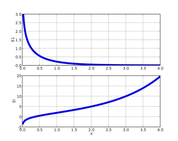
From the two series suggested in previous subsections, it follows that E 1 behaves like a negative exponential for large values of the argument and like a logarithm for small values. For positive real values of the argument, E 1 can be bracketed by elementary functions as follows:

1 2 e − x ln ( 1 + 2 x ) < E 1 ( x ) < e − x ln ( 1 + 1 x ) x > 0

The left-hand side of this inequality is shown in the graph to the left in blue; the central part E 1 ( x ) is shown in black and the right-hand side is shown in red.

Definition by Ein

Both Ei and E 1 can be written more simply using the entire function Ein defined as

Ein ⁡ ( z ) = ∫ 0 z ( 1 − e − t ) d t t = ∑ k = 1 ∞ ( − 1 ) k + 1 z k k k !

(note that this is just the alternating series in the above definition of E 1 ). Then we have

E 1 ( z ) = − γ − ln ⁡ z + E i n ( z ) | Arg ⁡ ( z ) | < π Ei ⁡ ( x ) = γ + ln ⁡ x − Ein ⁡ ( − x ) x > 0

Relation with other functions

Kummer's equation

z d 2 w d z 2 + ( b − z ) d w d z − a w = 0

is usually solved by the confluent hypergeometric functions M ( a , b , z ) and U ( a , b , z ) . But when a = 0 and b = 1 , that is,

z d 2 w d z 2 + ( 1 − z ) d w d z = 0

we have

M ( 0 , 1 , z ) = U ( 0 , 1 , z ) = 1

for all z. A second solution is then given by E₁(−z). In fact,

E 1 ( − z ) = − γ − i π + ∂ [ U ( a , 1 , z ) − M ( a , 1 , z ) ] ∂ a , 0 < A r g ( z ) < 2 π

with the derivative evaluated at a = 0. Another connexion with the confluent hypergeometric functions is that E₁ is an exponential times the function U(1,1,z):

E 1 ( z ) = e − z U ( 1 , 1 , z )

The exponential integral is closely related to the logarithmic integral function li(x) by the formula

li ⁡ ( e x ) = Ei ⁡ ( x )

for non-zero real values of x .

The exponential integral may also be generalized to

E n ( x ) = ∫ 1 ∞ e − x t t n d t ,

which can be written as a special case of the incomplete gamma function:

E n ( x ) = x n − 1 Γ ( 1 − n , x ) .

For more information on the properties of this function, refer to the more extensive article on the incomplete gamma function.

The generalized form is sometimes called the Misra function φ m ( x ) , defined as

φ m ( x ) = E − m ( x ) .

Including a logarithm defines the generalized integro-exponential function

E s j ( z ) = 1 Γ ( j + 1 ) ∫ 1 ∞ ( log ⁡ t ) j e − z t t s d t .

The indefinite integral:

Ei ⁡ ( a ⋅ b ) = ∬ e a b d a d b

is similar in form to the ordinary generating function for d ( n ) , the number of divisors of n :

∑ n = 1 ∞ d ( n ) x n = ∑ a = 1 ∞ ∑ b = 1 ∞ x a b

Derivatives

The derivatives of the generalised functions E n can be calculated by means of the formula

E n ′ ( z ) = − E n − 1 ( z ) ( n = 1 , 2 , 3 , … )

Note that the function E 0 is easy to evaluate (making this recursion useful), since it is just e − z / z .

Exponential integral of imaginary argument

If z is imaginary, it has a nonnegative real part, so we can use the formula

E 1 ( z ) = ∫ 1 ∞ e − t z t d t

to get a relation with the trigonometric integrals Si and Ci :

E 1 ( i x ) = i [ − 1 2 π + Si ⁡ ( x ) ] − Ci ⁡ ( x ) ( x > 0 )

The real and imaginary parts of E 1 ( i x ) are plotted in the figure to the right with black and red curves.

Approximations

There has been a number of approximations for the exponential integral function. These include

The Swamee and Ohija approximation

where A = ln ⁡ [ ( 0.56146 x + 0.65 ) ( 1 + x ) ] , and B = x 4 e 7.7 x ( 2 + x ) 3.7

The Allen and Hastings approximation

where a ≜ [ − 0.57722 , 0.99999 , − 0.24991 , 0.5519 , − 0.00976 , 0.00108 ] T , b ≜ [ 0.26777 , 8.63476 , 18.05902 , 8.57333 ] T , c ≜ [ 3.95850 , 21.0996525.63296 , 9.57332 ] T , and x k ≜ [ x 0 , x 1 , … , x k ] T .

The continued fraction expansion

The approximation of Barry et al.

where h = 1 1 + x x + h ∞ q 1 + q , q = 20 47 x 31 / 26 , h ∞ = ( 1 − G ) ( G 2 − 6 G + 12 ) 3 G ( 2 − G ) 2 b , b = 2 ( 1 − G ) G ( 2 − G ) , G = e − γ , where γ is Euler–Mascheroni constant.

Applications

Time-dependent heat transfer

Nonequilibrium groundwater flow in the Theis solution (called a well function)

Radiative transfer in stellar atmospheres

Radial diffusivity equation for transient or unsteady state flow with line sources and sinks

Solutions to the neutron transport equation in simplified 1-D geometries.