Euler spiral

Track transition curve

An object traveling on a circular path experiences a centripetal acceleration. When a vehicle traveling on a straight path suddenly transitions to a tangential circular path, it experiences a sudden centripetal acceleration starting at the tangent point; and this centripetal force acts instantly causing much discomfort (causing jerk).

On early railroads this instant application of lateral force was not an issue since low speeds and wide-radius curves were employed (lateral forces on the passengers and the lateral sway was small and tolerable). As speeds of rail vehicles increased over the years, it became obvious that an easement is necessary so that the centripetal acceleration increases linearly with the traveled distance. Given the expression of centripetal acceleration V² / R, the obvious solution is to provide an easement curve whose curvature, 1 / R, increases linearly with the traveled distance. This geometry is an Euler spiral.

Unaware of the solution of the geometry by Leonhard Euler, Rankine cited the cubic curve (a polynomial curve of degree 3), which is an approximation of the Euler spiral for small angular changes in the same way that a parabola is an approximation to a circular curve.

Marie Alfred Cornu (and later some civil engineers) also solved the calculus of Euler spiral independently. Euler spirals are now widely used in rail and highway engineering for providing a transition or an easement between a tangent and a horizontal circular curve.

Optics

The Cornu spiral can be used to describe a diffraction pattern.

Integrated optics

Bends with continuously varying radius of curvature following the Euler spiral are also used to reduce losses in photonic integrated circuits, either in singlemode waveguides, to smoothen the abrupt change of curvature and coupling to radiation modes, or in multimode waveguides, in order to suppress coupling to higher order modes and ensure effective singlemode operation. A pioneering and very elegant application of the Euler spiral to waveguides had been made as early as 1957, with a hollow metal waveguide for microwaves. There the idea was to exploit the fact that a straight metal waveguide can be physically bent to naturally take a gradual bend shape resembling an Euler spiral.

Auto Racing

Motorsport author Adam Brouillard has shown the Euler spiral's use in optimizing the racing line during the corner entry portion of a turn.

Expansion of Fresnel integral

If a = 1, which is the case for normalized Euler curve, then the Cartesian coordinates are given by Fresnel integrals (or Euler integrals):

C ( L ) = ∫ 0 L cos ⁡ ( s 2 ) d s S ( L ) = ∫ 0 L sin ⁡ ( s 2 ) d s

Expand C(L) according to power series expansion of cosine:

cos ⁡ θ = 1 − θ 2 2 ! + θ 4 4 ! − θ 6 6 ! + ⋯ C ( L ) = ∫ 0 L cos ⁡ ( s 2 ) d s = ∫ 0 L ( 1 − s 4 2 ! + s 8 4 ! − s 12 6 ! + ⋯ ) d s = L − L 5 5 × 2 ! + L 9 9 × 4 ! − L 13 13 × 6 ! + ⋯

Expand S(L) according to power series expansion of sine:

sin ⁡ θ = θ − θ 3 3 ! + θ 5 5 ! − θ 7 7 ! + ⋯ S ( L ) = ∫ 0 L sin ⁡ ( s 2 ) d s = ∫ 0 L ( s 2 − s 6 3 ! + s 10 5 ! − s 14 7 ! + ⋯ ) d s = L 3 3 − L 7 7 × 3 ! + L 11 11 × 5 ! − L 15 15 × 7 ! + ⋯

Normalization and conclusion

For a given Euler curve with:

2 R L = 2 R c L s = 1 a 2

or

1 R = L R c L s = 2 a 2 L

then

x = 1 a ∫ 0 L ′ cos ⁡ s 2 d s y = 1 a ∫ 0 L ′ sin ⁡ s 2 d s

where L ′ = a L and a = 1 2 R c L s .

The process of obtaining solution of (x, y) of an Euler spiral can thus be described as:

Map L of the original Euler spiral by multiplying with factor a to L′ of the normalized Euler spiral;

Find (x′, y′) from the Fresnel integrals; and

Map (x′, y′) to (x, y) by scaling up (denormalize) with factor 1 / a . Note that 1 / a > 1 .

In the normalization process,

R c ′ = R c 2 R c L s = R c 2 L s L s ′ = L s 2 R c L s = L s 2 R c

Then

2 R c ′ L s ′ = 2 R c 2 L s L s 2 R c = 2 2 = 1

Generally the normalization reduces L' to a small value (<1) and results in good converging characteristics of the Fresnel integral manageable with only a few terms (at a price of increased numerical instability of the calculation, esp. for bigger θ values.).

Illustration

Given:

R c = 300 m L s = 100 m

Then

θ s = L s 2 R c = 100 2 × 300 = 0.1667   radian

And

2 R c L s = 60 , 000

We scale down the Euler spiral by √60,000, i.e.100√6 to normalized Euler spiral that has:

R c ′ = 3 6 m L s ′ = 1 6 m 2 R c ′ L s ′ = 2 × 3 6 × 1 6 = 1

And

θ s = L s ′ 2 R c ′ = 1 6 2 × 3 6 = 0.1667   radian

The two angles θ s are the same. This thus confirms that the original and normalized Euler spirals are geometrically similar. The locus of the normalized curve can be determined from Fresnel Integral, while the locus of the original Euler spiral can be obtained by scaling back / up or denormalizing.

Other properties of normalized Euler spirals

Normalized Euler spirals can be expressed as:

x = ∫ 0 L cos ⁡ s 2 d s y = ∫ 0 L sin ⁡ s 2 d s

Or expressed as power series:

x = ∑ i = 0 ∞ ( − 1 ) i ( 2 i ) ! s 4 i + 1 4 i + 1 | 0 L = ∑ i = 0 ∞ ( − 1 ) i ( 2 i ) ! L 4 i + 1 4 i + 1 y = ∑ i = 0 ∞ ( − 1 ) i ( 2 i + 1 ) ! s 4 i + 3 4 i + 3 | 0 L = ∑ i = 0 ∞ ( − 1 ) i ( 2 i + 1 ) ! L 4 i + 3 4 i + 3

The normalized Euler spiral will converge to a single point in the limit, which (noting that L = s ) can be expressed as:

x ′ = lim s → ∞ ∫ 0 L cos ⁡ ( s 2 ) d s = 1 2 π 2 y ′ = lim s → ∞ ∫ 0 L sin ⁡ ( s 2 ) d s = 1 2 π 2

Normalized Euler spirals have the following properties:

2 R c L s = 1 θ s = L s 2 R c = L s 2

And

θ = θ s ⋅ L 2 L s 2 = L 2 1 R = d θ d L = 2 L

Note that 2 R c L s = 1 also means 1 / R c = 2 L s , in agreement with the last mathematical statement.

Code for producing an Euler spiral

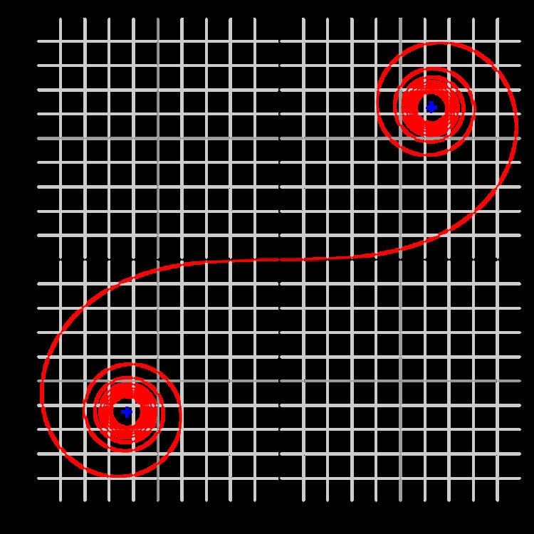
The following SageMath code produces the second graph above. The first four lines express the Euler spiral component. Fresnel functions could not be found. Instead, the integrals of two expanded Taylor series are adopted. The remaining code expresses respectively the tangent and the circle, including the computation for the center coordinates.

The following is Mathematica code for the Euler spiral component (it works directly in wolframalpha.com):

The following is Xcas code for the Euler spiral component:

plotparam([int(cos(u^2),u,0,t),int(sin(u^2),u,0,t)],t,-4,4)

The following is SageMath code for the complete double ended Euler spiral:

The following is JavaScript code for drawing an Euler spiral on a canvas element: