Fresnel integral - Alchetron, The Free Social Encyclopedia

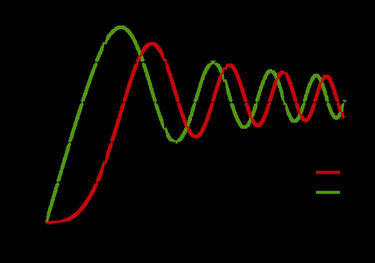
Fresnel integrals, S(x) and C(x), are two transcendental functions named after Augustin-Jean Fresnel that are used in optics, which are closely related to the error function (erf). They arise in the description of near-field Fresnel diffraction phenomena and are defined through the following integral representations:

Definition

The Fresnel integrals admit the following power series expansions that converge for all x:

S ( x ) = ∫ 0 x sin ⁡ ( t 2 ) d t = ∑ n = 0 ∞ ( − 1 ) n x 4 n + 3 ( 2 n + 1 ) ! ( 4 n + 3 ) C ( x ) = ∫ 0 x cos ⁡ ( t 2 ) d t = ∑ n = 0 ∞ ( − 1 ) n x 4 n + 1 ( 2 n ) ! ( 4 n + 1 )

Some authors, including Abramowitz and Stegun, (eqs 7.3.1 – 7.3.2) use π 2 t 2 for the argument of the integrals defining S(x) and C(x). To get these functions, multiply the above integrals by 2 π and multiply the argument x by π 2 .

Euler spiral

The Euler spiral, also known as Cornu spiral or clothoid, is the curve generated by a parametric plot of S ( t ) against C ( t ) . The Cornu spiral was created by Marie Alfred Cornu as a nomogram for diffraction computations in science and engineering.

From the definitions of Fresnel integrals, the infinitesimals d x and d y are thus:

d x = C ′ ( t ) d t = cos ⁡ ( t 2 ) d t , d y = S ′ ( t ) d t = sin ⁡ ( t 2 ) d t .

Thus the length of the spiral measured from the origin can be expressed as

L = ∫ 0 t 0 d x 2 + d y 2 = ∫ 0 t 0 d t = t 0 .

That is, the parameter t is the curve length measured from the origin ( 0 , 0 ) , and the Euler spiral has infinite length. The vector ( cos ⁡ ( t 2 ) , sin ⁡ ( t 2 ) ) also expresses the unit tangent vector along the spiral, giving θ = t 2 . Since t is the curve length, the curvature κ can be expressed as

κ = 1 R = d θ d t = 2 t .

And the rate of change of curvature with respect to the curve length is

d κ d t = d 2 θ d t 2 = 2.

An Euler spiral has the property that its curvature at any point is proportional to the distance along the spiral, measured from the origin. This property makes it useful as a transition curve in highway and railway engineering.

If a vehicle follows the spiral at unit speed, the parameter t in the above derivatives also represents the time. That is, a vehicle following the spiral at constant speed will have a constant rate of angular acceleration.

Sections from Euler spirals are commonly incorporated into the shape of roller-coaster loops to make what are known as clothoid loops.

Properties

C(x) and S(x) are odd functions of x.

Asymptotics of the Fresnel integrals as x → ∞ are given by the formulas:

Using the power series expansions above, the Fresnel integrals can be extended to the domain of complex numbers, and they become analytic functions of a complex variable.

The Fresnel integrals can be expressed using the error function as follows:

or

C and S are entire functions.

Limits as x approaches infinity

The integrals defining C(x) and S(x) cannot be evaluated in the closed form in terms of elementary functions, except in special cases. The limits of these functions as x goes to infinity are known:

The limits of C and S as the argument tends to infinity can be found by the methods of complex analysis. This uses the contour integral of the function

e − t 2

around the boundary of the sector-shaped region in the complex plane formed by the positive x-axis, the bisector of the first quadrant y = x with x ≥ 0, and a circular arc of radius R centered at the origin.

As R goes to infinity, the integral along the circular arc tends to 0, the integral along the real axis tends to the half Gaussian integral

∫ 0 ∞ e − t 2 d t = π 2 .

Note too that because the integrand is an entire function on the complex plane, its integral along the whole contour is zero. Overall, we must have

∫ 0 ∞ e − t 2 d t = ∫ γ 3 e − t 2 d t

where γ 3 denotes the bisector of the first quadrant, as in the diagram. To evaluate the right hand side, parametrize the bisector as t = r e π i / 4 = 2 2 ( 1 + i ) r where r ranges from 0 to + ∞ . Note that the square of this expression is just + i r 2 . Therefore, substitution gives the right hand side as

∫ 0 ∞ e − i r 2 2 2 ( 1 + i ) d r .

Using Euler's formula to take real and imaginary parts of e − i r 2 gives this as

∫ 0 ∞ ( cos ⁡ ( r 2 ) − i sin ⁡ ( r 2 ) ) 2 2 ( 1 + i ) d r = 2 2 ∫ 0 ∞ [ cos ⁡ ( r 2 ) + sin ⁡ ( r 2 ) ] + [ cos ⁡ ( r 2 ) − sin ⁡ ( r 2 ) ] i d r = π 2 + 0 i

where we have written 0 i to emphasize that the original Gaussian integral's value is completely real with zero imaginary part. Letting I C = ∫ 0 ∞ cos ⁡ ( r 2 ) d r , I S = ∫ 0 ∞ sin ⁡ ( r 2 ) d r and then equating real and imaginary parts produces the following system of two equations in the two unknowns I C , I S :

I C + I S = π 2 , I C − I S = 0.

Solving this for I C and I S gives the desired result.

Generalization

The integral

∫ x m exp ⁡ ( i x n ) d x = ∫ ∑ l = 0 ∞ i l x m + n l l ! d x = ∑ l = 0 ∞ i l ( m + n l + 1 ) x m + n l + 1 l !

is a confluent hypergeometric function and also an incomplete Gamma function

∫ x m exp ⁡ ( i x n ) d x = x m + 1 m + 1 1 F 1 ( m + 1 n 1 + m + 1 n ∣ i x n ) = 1 n i ( m + 1 ) / n γ ( m + 1 n , − i x n ) ,

which reduces to Fresnel integrals if real or imaginary parts are taken:

∫ x m sin ⁡ ( x n ) d x = x m + n + 1 m + n + 1 1 F 2 ( 1 2 + m + 1 2 n 3 2 + m + 1 2 n , 3 2 ∣ − x 2 n 4 ) .

The leading term in the asymptotic expansion is

1 F 1 ( m + 1 n 1 + m + 1 n ∣ i x n ) ∼ m + 1 n Γ ( m + 1 n ) e i π ( m + 1 ) / ( 2 n ) x − m − 1 ,

and therefore

∫ 0 ∞ x m exp ⁡ ( i x n ) d x = 1 n Γ ( m + 1 n ) e i π ( m + 1 ) / ( 2 n ) .

For m = 0, the imaginary part of this equation in particular is

∫ 0 ∞ sin ⁡ ( x a ) d x = Γ ( 1 + 1 a ) sin ⁡ ( π 2 a )

with the left-hand side converging for a > 1 and the right-hand side being its analytical extension to the whole plane less where lie the poles of Γ ( a − 1 ) .

The Kummer transformation of the confluent hypergeometric function is

∫ x m exp ⁡ ( i x n ) d x = V n , m ( x ) e i x n

with

V n , m := x m + 1 m + 1 1 F 1 ( 1 1 + m + 1 n ∣ − i x n ) .

Applications

The Fresnel integrals were originally used in the calculation of the electromagnetic field intensity in an environment where light bends around opaque objects. More recently, they have been used in the design of highways and railways, specifically their curvature transition zones, see track transition curve. Another application is roller coasters. Another application is for calculating the transitions on a velodrome track to allow rapid entry to the bends and gradual exit.

References

Fresnel integral Wikipedia

(Text) CC BY-SA

Contents