
 | ||
In mathematics, physics and engineering, the cardinal sine function or sinc function, denoted by sinc(x), has two slightly different definitions.
Contents
- Properties
- Relationship to the Dirac delta distribution
- Summation
- Series expansion
- Higher dimensions
- References
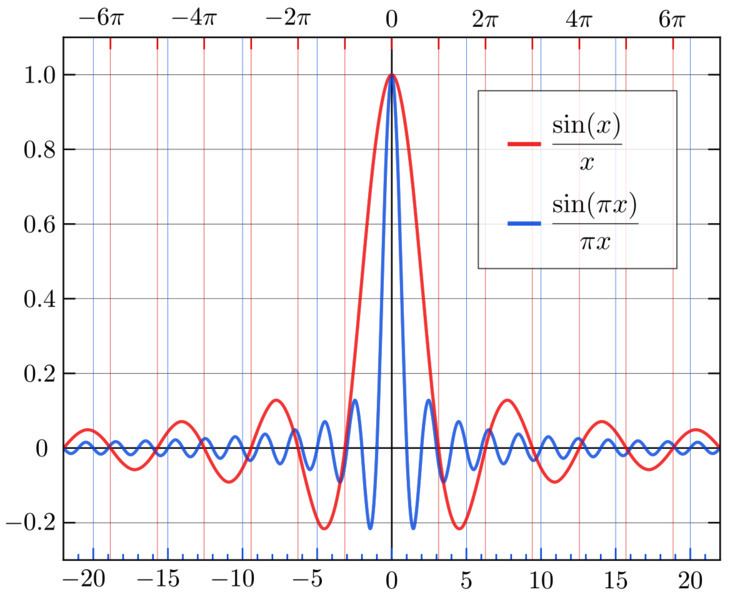
In mathematics, the historical unnormalized sinc function is defined for x ≠ 0 by
In digital signal processing and information theory, the normalized sinc function is commonly defined for x ≠ 0 by
In either case, the value at x = 0 is defined to be the limiting value sinc(0) = 1.
The normalization causes the definite integral of the function over the real numbers to equal 1 (whereas the same integral of the unnormalized sinc function has a value of π). As a further useful property, all of the zeros of the normalized sinc function are integer values of x.
The normalized sinc function is the Fourier transform of the rectangular function with no scaling. It is used in the concept of reconstructing a continuous bandlimited signal from uniformly spaced samples of that signal.
The only difference between the two definitions is in the scaling of the independent variable (the x-axis) by a factor of π. In both cases, the value of the function at the removable singularity at zero is understood to be the limit value 1. The sinc function is then analytic everywhere and hence an entire function.
The term sinc /ˈsɪŋk/ is a contraction of the function's full Latin name, the sinus cardinalis (cardinal sine). It was introduced by Phillip M. Woodward in his 1952 paper "Information theory and inverse probability in telecommunication", in which he said the function "occurs so often in Fourier analysis and its applications that it does seem to merit some notation of its own", and his 1953 book Probability and Information Theory, with Applications to Radar.
Properties
The zero crossings of the unnormalized sinc are at non-zero integer multiples of π, while zero crossings of the normalized sinc occur at non-zero integers.
The local maxima and minima of the unnormalized sinc correspond to its intersections with the cosine function. That is, sin(ξ)/ξ = cos(ξ) for all points ξ where the derivative of sin(x)/x is zero and thus a local extremum is reached.
A good approximation of the x-coordinate of the nth extremum with positive x-coordinate is
where odd n lead to a local minimum and even n to a local maximum. Because of symmetry around the y-axis, there exist extrema with x-coordinates −xn. In addition, there is an absolute maximum at ξ0 = (0,1).
The normalized sinc function has a simple representation as the infinite product
and is related to the gamma function Γ(x) through Euler's reflection formula,
Euler discovered that
The continuous Fourier transform of the normalized sinc (to ordinary frequency) is rect( f ),
where the rectangular function is 1 for argument between −1/2 and 1/2, and zero otherwise. This corresponds to the fact that the sinc filter is the ideal (brick-wall, meaning rectangular frequency response) low-pass filter.
This Fourier integral, including the special case
is an improper integral (cf. Dirichlet integral) and not a convergent Lebesgue integral, as
The normalized sinc function has properties that make it ideal in relationship to interpolation of sampled bandlimited functions:
Other properties of the two sinc functions include:
Relationship to the Dirac delta distribution
The normalized sinc function can be used as a nascent delta function, meaning that the following weak limit holds,
This is not an ordinary limit, since the left side does not converge. Rather, it means that
for any smooth function φ(x) with compact support.
In the above expression, as a → 0, the number of oscillations per unit length of the sinc function approaches infinity. Nevertheless, the expression always oscillates inside an envelope of ±1/πx, regardless of the value of a.
This complicates the informal picture of δ(x) as being zero for all x except at the point x = 0, and illustrates the problem of thinking of the delta function as a function rather than as a distribution. A similar situation is found in the Gibbs phenomenon.
Summation
All sums in this section refer to the unnormalized sinc function.
The sum of sinc(n) over integer n from 1 to ∞ equals π − 1/2.
The sum of the squares also equals π − 1/2.
When the signs of the addends alternate and begin with +, the sum equals 1/2.
The alternating sums of the squares and cubes also equal 1/2.
Series expansion
Unnormalized sinc(x):
Higher dimensions
The product of 1-D sinc functions readily provides a multivariate sinc function for the square, Cartesian, grid (lattice): sincC(x, y) = sinc(x)sinc(y) whose Fourier transform is the indicator function of a square in the frequency space (i.e., the brick wall defined in 2-D space). The sinc function for a non-Cartesian lattice (e.g., hexagonal lattice) is a function whose Fourier transform is the indicator function of the Brillouin zone of that lattice. For example, the sinc function for the hexagonal lattice is a function whose Fourier transform is the indicator function of the unit hexagon in the frequency space. For a non-Cartesian lattice this function can not be obtained by a simple tensor-product. However, the explicit formula for the sinc function for the hexagonal, body centered cubic, face centered cubic and other higher-dimensional lattices can be explicitly derived using the geometric properties of Brillouin zones and their connection to zonotopes.
For example, a hexagonal lattice can be generated by the (integer) linear span of the vectors
Denoting
one can derive the sinc function for this hexagonal lattice as:
This construction can be used to design Lanczos window for general multidimensional lattices.