Protein structure prediction

Protein structure and terminology

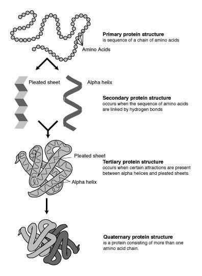
Proteins are chains of amino acids joined together by peptide bonds. Many conformations of this chain are possible due to the rotation of the chain about each Cα atom. It is these conformational changes that are responsible for differences in the three dimensional structure of proteins. Each amino acid in the chain is polar, i.e. it has separated positive and negative charged regions with a free C=O group, which can act as hydrogen bond acceptor and an NH group, which can act as hydrogen bond donor. These groups can therefore interact in the protein structure. The 20 amino acids can be classified according to the chemistry of the side chain which also plays an important structural role. Glycine takes on a special position, as it has the smallest side chain, only one Hydrogen atom, and therefore can increase the local flexibility in the protein structure. Cysteine on the other hand can react with another cysteine residue and thereby form a cross link stabilizing the whole structure.

The protein structure can be considered as a sequence of secondary structure elements, such as α helices and β sheets, which together constitute the overall three-dimensional configuration of the protein chain. In these secondary structures regular patterns of H bonds are formed between neighboring amino acids, and the amino acids have similar Φ and Ψ angles.

The formation of these structures neutralizes the polar groups on each amino acid. The secondary structures are tightly packed in the protein core in a hydrophobic environment. Each amino acid side group has a limited volume to occupy and a limited number of possible interactions with other nearby side chains, a situation that must be taken into account in molecular modeling and alignments.

α Helix

The α helix is the most abundant type of secondary structure in proteins. The α helix has 3.6 amino acids per turn with an H bond formed between every fourth residue; the average length is 10 amino acids (3 turns) or 10 Å but varies from 5 to 40 (1.5 to 11 turns). The alignment of the H bonds creates a dipole moment for the helix with a resulting partial positive charge at the amino end of the helix. Because this region has free NH2 groups, it will interact with negatively charged groups such as phosphates. The most common location of α helices is at the surface of protein cores, where they provide an interface with the aqueous environment. The inner-facing side of the helix tends to have hydrophobic amino acids and the outer-facing side hydrophilic amino acids. Thus, every third of four amino acids along the chain will tend to be hydrophobic, a pattern that can be quite readily detected. In the leucine zipper motif, a repeating pattern of leucines on the facing sides of two adjacent helices is highly predictive of the motif. A helical-wheel plot can be used to show this repeated pattern. Other α helices buried in the protein core or in cellular membranes have a higher and more regular distribution of hydrophobic amino acids, and are highly predictive of such structures. Helices exposed on the surface have a lower proportion of hydrophobic amino acids. Amino acid content can be predictive of an α -helical region. Regions richer in alanine (A), glutamic acid (E), leucine (L), and methionine (M) and poorer in proline (P), glycine (G), tyrosine (Y), and serine (S) tend to form an α helix. Proline destabilizes or breaks an α helix but can be present in longer helices, forming a bend.

β sheet

β sheets are formed by H bonds between an average of 5–10 consecutive amino acids in one portion of the chain with another 5–10 farther down the chain. The interacting regions may be adjacent, with a short loop in between, or far apart, with other structures in between. Every chain may run in the same direction to form a parallel sheet, every other chain may run in the reverse chemical direction to form an anti parallel sheet, or the chains may be parallel and anti parallel to form a mixed sheet.The pattern of H bonding is different in the parallel and anti parallel configurations. Each amino acid in the interior strands of the sheet forms two H bonds with neighboring amino acids, whereas each amino acid on the outside strands forms only one bond with an interior strand. Looking across the sheet at right angles to the strands, more distant strands are rotated slightly counterclockwise to form a left-handed twist. The Cα atoms alternate above and below the sheet in a pleated structure, and the R side groups of the amino acids alternate above and below the pleats. The Φ and Ψ angles of the amino acids in sheets vary considerably in one region of the Ramachandran plot. It is more difficult to predict the location of β sheets than of α helices. The situation improves somewhat when the amino acid variation in multiple sequence alignments is taken into account.

Loop

Loops are regions of a protein chain that are (1) between α helices and β sheets, (2) of various lengths and three-dimensional configurations, and (3) on the surface of the structure. Hairpin loops that represent a complete turn in the polypeptide chain joining two antiparallel β strands may be as short as two amino acids in length. Loops interact with the surrounding aqueous environment and other proteins. Because amino acids in loops are not constrained by space and environment as are amino acids in the core region, and do not have an effect on the arrangement of secondary structures in the core, more substitutions, insertions, and deletions may occur. Thus, in a sequence alignment, the presence of these features may be an indication of a loop. The positions of introns in genomic DNA sometimes correspond to the locations of loops in the encoded protein. Loops also tend to have charged and polar amino acids and are frequently a component of active sites. A detailed examination of loop structures has shown that they fall into distinct families.

Coils

A region of secondary structure that is not a α helix, a β sheet, or a recognizable turn is commonly referred to as a coil.

Protein classification

Proteins may be classified according to both structural and sequence similarity. For structural classification, the sizes and spatial arrangements of secondary structures described in the above paragraph are compared in known three-dimensional structures.Classification based on sequence similarity was historically the first to be used. Initially, similarity based on alignments of whole sequences was performed. Later, proteins were classified on the basis of the occurrence of conserved amino acid patterns. Databases that classify proteins by one or more of these schemes are available. In considering protein classification schemes, it is important to keep several observations in mind. First, two entirely different protein sequences from different evolutionary origins may fold into a similar structure. Conversely, the sequence of an ancient gene for a given structure may have diverged considerably in different species while at the same time maintaining the same basic structural features. Recognizing any remaining sequence similarity in such cases may be a very difficult task. Second, two proteins that share a significant degree of sequence similarity either with each other or with a third sequence also share an evolutionary origin and should share some structural features also. However, gene duplication and genetic rearrangements during evolution may give rise to new gene copies, which can then evolve into proteins with new function and structure.

Terms Used for Classifying Protein Structures and Sequences

The more commonly used terms for evolutionary and structural relationships among proteins are listed below. Many additional terms are used for various kinds of structural features found in proteins. Descriptions of such terms may be found at the CATH Web site the Structural Classification of Proteins (SCOP) Web site and a Glaxo-Wellcome tutorial on the Swiss bioinformatics Expasy Web site.

active site 

a localized combination of amino acid side groups within the tertiary (three-dimensional) or quaternary (protein subunit) structure that can interact with a chemically specific substrate and that provides the protein with biological activity. Proteins of very different amino acid sequences may fold into a structure that produces the same active site.

architecture 

the relative orientations of secondary structures in a three-dimensional structure without regard to whether or not they share a similar loop structure.

fold 

a type of architecture that also has a conserved loop structure.

blocks 

a conserved amino acid sequence pattern in a family of proteins. The pattern includes a series of possible matches at each position in the represented sequences, but there are not any inserted or deleted positions in the pattern or in the sequences. By way of contrast, sequence profiles are a type of scoring matrix that represents a similar set of patterns that includes insertions and deletions.

class 

a term used to classify protein domains according to their secondary structural content and organization. Four classes were originally recognized by Levitt and Chothia (1976), and several others have been added in the SCOP database. Three classes are given in the CATH database: mainly-α, mainly-β, and α–β, with the α–β class including both alternating α/β and α+β structures.

core 

the portion of a folded protein molecule that comprises the hydrophobic interior of α-helices and β-sheets. The compact structure brings together side groups of amino acids into close enough proximity so that they can interact. When comparing protein structures, as in the SCOP database, core is the region common to most of the structures that share a common fold or that are in the same superfamily. In structure prediction, core is sometimes defined as the arrangement of secondary structures that is likely to be conserved during evolutionary change.

domain (sequence context) 

a segment of a polypeptide chain that can fold into a three-dimensional structure irrespective of the presence of other segments of the chain. The separate domains of a given protein may interact extensively or may be joined only by a length of polypeptide chain. A protein with several domains may use these domains for functional interactions with different molecules.

family (sequence context) 

a group of proteins of similar biochemical function that are more than 50% identical when aligned. This same cutoff is still used by the Protein Information Resource (PIR). A protein family comprises proteins with the same function in different organisms (orthologous sequences) but may also include proteins in the same organism (paralogous sequences) derived from gene duplication and rearrangements. If a multiple sequence alignment of a protein family reveals a common level of similarity throughout the lengths of the proteins, PIR refers to the family as a homeomorphic family. The aligned region is referred to as a homeomorphic domain, and this region may comprise several smaller homology domains that are shared with other families. Families may be further subdivided into subfamilies or grouped into superfamilies based on respective higher or lower levels of sequence similarity. The SCOP database reports 1296 families and the CATH database (version 1.7 beta), reports 1846 families.When the sequences of proteins with the same function are examined in greater detail, some are found to share high sequence similarity. They are obviously members of the same family by the above criteria. However, others are found that have very little, or even insignificant, sequence similarity with other family members. In such cases, the family relationship between two distant family members A and C can often be demonstrated by finding an additional family member B that shares significant similarity with both A and C. Thus, B provides a connecting link between A and C. Another approach is to examine distant alignments for highly conserved matches.At a level of identity of 50%, proteins are likely to have the same three-dimensional structure, and the identical atoms in the sequence alignment will also superimpose within approximately 1 Å in the structural model. Thus, if the structure of one member of a family is known, a reliable prediction may be made for a second member of the family, and the higher the identity level, the more reliable the prediction. Protein structural modeling can be performed by examining how well the amino acid substitutions fit into the core of the three-dimensional structure.

family (structural context) 

as used in the FSSP database (Families of structurally similar proteins) and the DALI/FSSP Web site, two structures that have a significant level of structural similarity but not necessarily significant sequence similarity.

fold 

similar to structural motif, includes a larger combination of secondary structural units in the same configuration. Thus, proteins sharing the same fold have the same combination of secondary structures that are connected by similar loops. An example is the Rossman fold comprising several alternating α helices and parallel β strands. In the SCOP, CATH, and FSSP databases, the known protein structures have been classified into hierarchical levels of structural complexity with the fold as a basic level of classification.

homologous domain (sequence context) 

an extended sequence pattern, generally found by sequence alignment methods, that indicates a common evolutionary origin among the aligned sequences. A homology domain is generally longer than motifs. The domain may include all of a given protein sequence or only a portion of the sequence. Some domains are complex and made up of several smaller homology domains that became joined to form a larger one during evolution. A domain that covers an entire sequence is called the homeomorphic domain by PIR (Protein Information Resource).

module 

a region of conserved amino acid patterns comprising one or more motifs and considered to be a fundamental unit of structure or function. The presence of a module has also been used to classify proteins into families.

motif (sequence context) 

a conserved pattern of amino acids that is found in two or more proteins. In the Prosite catalog, a motif is an amino acid pattern that is found in a group of proteins that have a similar biochemical activity, and that often is near the active site of the protein. Examples of sequence motif databases are the Prosite catalog and the Stanford Motifs Database.

motif (structural context) 

a combination of several secondary structural elements produced by the folding of adjacent sections of the polypeptide chain into a specific three-dimensional configuration. An example is the helix-loop-helix motif. Structural motifs are also referred to as supersecondary structures and folds.

position-specific scoring matrix (sequence context, also known as weight or scoring matrix) 

represents a conserved region in a multiple sequence alignment with no gaps. Each matrix column represents the variation found in one column of the multiple sequence alignment.Position-specific scoring matrix—3D (structural context) represents the amino acid variation found in an alignment of proteins that fall into the same structural class. Matrix columns represent the amino acid variation found at one amino acid position in the aligned structures.

primary structure 

the linear amino acid sequence of a protein, which chemically is a polypeptide chain composed of amino acids joined by peptide bonds.

profile (sequence context) 

a scoring matrix that represents a multiple sequence alignment of a protein family. The profile is usually obtained from a well-conserved region in a multiple sequence alignment. The profile is in the form of a matrix with each column representing a position in the alignment and each row one of the amino acids. Matrix values give the likelihood of each amino acid at the corresponding position in the alignment. The profile is moved along the target sequence to locate the best scoring regions by a dynamic programming algorithm. Gaps are allowed during matching and a gap penalty is included in this case as a negative score when no amino acid is matched. A sequence profile may also be represented by a hidden Markov model, referred to as a profile HMM.

profile (structural context) 

a scoring matrix that represents which amino acids should fit well and which should fit poorly at sequential positions in a known protein structure. Profile columns represent sequential positions in the structure, and profile rows represent the 20 amino acids. As with a sequence profile, the structural profile is moved along a target sequence to find the highest possible alignment score by a dynamic programming algorithm. Gaps may be included and receive a penalty. The resulting score provides an indication as to whether or not the target protein might adopt such a structure.

quaternary structure 

the three-dimensional configuration of a protein molecule comprising several independent polypeptide chains.

secondary structure 

the interactions that occur between the C, O, and NH groups on amino acids in a polypeptide chain to form α-helices, β-sheets, turns, loops, and other forms, and that facilitate the folding into a three-dimensional structure.

superfamily 

a group of protein families of the same or different lengths that are related by distant yet detectable sequence similarity. Members of a given superfamily thus have a common evolutionary origin. Originally, Dayhoff defined the cutoff for superfamily status as being the chance that the sequences are not related of 10 6, on the basis of an alignment score (Dayhoff et al. 1978). Proteins with few identities in an alignment of the sequences but with a convincingly common number of structural and functional features are placed in the same superfamily. At the level of three-dimensional structure, superfamily proteins will share common structural features such as a common fold, but there may also be differences in the number and arrangement of secondary structures. The PIR resource uses the term homeomorphic superfamilies to refer to superfamilies that are composed of sequences that can be aligned from end to end, representing a sharing of single sequence homology domain, a region of similarity that extends throughout the alignment. This domain may also comprise smaller homology domains that are shared with other protein families and superfamilies. Although a given protein sequence may contain domains found in several superfamilies, thus indicating a complex evolutionary history, sequences will be assigned to only one homeomorphic superfamily based on the presence of similarity throughout a multiple sequence alignment. The superfamily alignment may also include regions that do not align either within or at the ends of the alignment. In contrast, sequences in the same family align well throughout the alignment.

supersecondary structure 

a term with similar meaning to a structural motif. Tertiary structure is the three-dimensional or globular structure formed by the packing together or folding of secondary structures of a polypeptide chain.

Secondary structure

Secondary structure prediction is a set of techniques in bioinformatics that aim to predict the local secondary structures of proteins based only on knowledge of their amino acid sequence. For proteins, a prediction consists of assigning regions of the amino acid sequence as likely alpha helices, beta strands (often noted as "extended" conformations), or turns. The success of a prediction is determined by comparing it to the results of the DSSP algorithm (or similar e.g. STRIDE) applied to the crystal structure of the protein. Specialized algorithms have been developed for the detection of specific well-defined patterns such as transmembrane helices and coiled coils in proteins.

The best modern methods of secondary structure prediction in proteins reach about 80% accuracy; this high accuracy allows the use of the predictions as feature improving fold recognition and ab initio protein structure prediction, classification of structural motifs, and refinement of sequence alignments. The accuracy of current protein secondary structure prediction methods is assessed in weekly benchmarks such as LiveBench and EVA.

Background

Early methods of secondary structure prediction, introduced in the 1960s and early 1970s, focused on identifying likely alpha helices and were based mainly on helix-coil transition models. Significantly more accurate predictions that included beta sheets were introduced in the 1970s and relied on statistical assessments based on probability parameters derived from known solved structures. These methods, applied to a single sequence, are typically at most about 60-65% accurate, and often underpredict beta sheets. The evolutionary conservation of secondary structures can be exploited by simultaneously assessing many homologous sequences in a multiple sequence alignment, by calculating the net secondary structure propensity of an aligned column of amino acids. In concert with larger databases of known protein structures and modern machine learning methods such as neural nets and support vector machines, these methods can achieve up 80% overall accuracy in globular proteins. The theoretical upper limit of accuracy is around 90%, partly due to idiosyncrasies in DSSP assignment near the ends of secondary structures, where local conformations vary under native conditions but may be forced to assume a single conformation in crystals due to packing constraints. Limitations are also imposed by secondary structure prediction's inability to account for tertiary structure; for example, a sequence predicted as a likely helix may still be able to adopt a beta-strand conformation if it is located within a beta-sheet region of the protein and its side chains pack well with their neighbors. Dramatic conformational changes related to the protein's function or environment can also alter local secondary structure.

Historical perspective

To date, over 20 different secondary structure prediction methods have been developed. One of the first algorithms was Chou-Fasman method, which relies predominantly on probability parameters determined from relative frequencies of each amino acid's appearance in each type of secondary structure. The original Chou-Fasman parameters, determined from the small sample of structures solved in the mid-1970s, produce poor results compared to modern methods, though the parameterization has been updated since it was first published. The Chou-Fasman method is roughly 50-60% accurate in predicting secondary structures.

The next notable program was the GOR method, named for the three scientists who developed it — Garnier, Osguthorpe, and Robson, is an information theory-based method. It uses the more powerful probabilistic technique of Bayesian inference. The GOR method takes into account not only the probability of each amino acid having a particular secondary structure, but also the conditional probability of the amino acid assuming each structure given the contributions of its neighbors (it does not assume that the neighbors have that same structure). The approach is both more sensitive and more accurate than that of Chou and Fasman because amino acid structural propensities are only strong for a small number of amino acids such as proline and glycine. Weak contributions from each of many neighbors can add up to strong effects overall. The original GOR method was roughly 65% accurate and is dramatically more successful in predicting alpha helices than beta sheets, which it frequently mispredicted as loops or disorganized regions.

Another big step forward, was using machine learning methods. First artificial neural networks methods were used. As a training sets they use solved structures to identify common sequence motifs associated with particular arrangements of secondary structures. These methods are over 70% accurate in their predictions, although beta strands are still often underpredicted due to the lack of three-dimensional structural information that would allow assessment of hydrogen bonding patterns that can promote formation of the extended conformation required for the presence of a complete beta sheet. PSIPRED and JPRED are some of the most known programs based on neural networks for protein secondary structure prediction. Next, support vector machines have proven particularly useful for predicting the locations of turns, which are difficult to identify with statistical methods.

Extensions of machine learning techniques attempt to predict more fine-grained local properties of proteins, such as backbone dihedral angles in unassigned regions. Both SVMs and neural networks have been applied to this problem. More recently, real-value torsion angles can be accurately predicted by SPINE-X and successfully employed for ab initio structure prediction.

Other improvements

It is reported that in addition to the protein sequence, secondary structure formation depends on other factors. For example, it is reported that secondary structure tendencies depend also on local environment, solvent accessibility of residues, protein structural class, and even the organism from which the proteins are obtained. Based on such observations, some studies have shown that secondary structure prediction can be improved by addition of information about protein structural class, residue accessible surface area and also contact number information.

Tertiary structure

The practical role of protein structure prediction is now more important than ever. Massive amounts of protein sequence data are produced by modern large-scale DNA sequencing efforts such as the Human Genome Project. Despite community-wide efforts in structural genomics, the output of experimentally determined protein structures—typically by time-consuming and relatively expensive X-ray crystallography or NMR spectroscopy—is lagging far behind the output of protein sequences.

The protein structure prediction remains an extremely difficult and unresolved undertaking. The two main problems are calculation of protein free energy and finding the global minimum of this energy. A protein structure prediction method must explore the space of possible protein structures which is astronomically large. These problems can be partially bypassed in "comparative" or homology modeling and fold recognition methods, in which the search space is pruned by the assumption that the protein in question adopts a structure that is close to the experimentally determined structure of another homologous protein. On the other hand, the de novo or ab initio protein structure prediction methods must explicitly resolve these problems. The progress and challenges in protein structure prediction has been reviewed in Zhang 2008.

Energy- and fragment-based methods

Ab initio- or de novo- protein modelling methods seek to build three-dimensional protein models "from scratch", i.e., based on physical principles rather than (directly) on previously solved structures. There are many possible procedures that either attempt to mimic protein folding or apply some stochastic method to search possible solutions (i.e., global optimization of a suitable energy function). These procedures tend to require vast computational resources, and have thus only been carried out for tiny proteins. To predict protein structure de novo for larger proteins will require better algorithms and larger computational resources like those afforded by either powerful supercomputers (such as Blue Gene or MDGRAPE-3) or distributed computing (such as Folding@home, the Human Proteome Folding Project and Rosetta@Home). Although these computational barriers are vast, the potential benefits of structural genomics (by predicted or experimental methods) make ab initio structure prediction an active research field.

As of 2009, a 50-residue protein could be simulated atom-by-atom on a supercomputer for 1 millisecond. As of 2012, comparable stable-state sampling could be done on a standard desktop with a new graphics card and more sophisticated algorithms. A much larger simulation timescales can be achieved using coarse-grained modeling.

Evolutionary covariation to predict 3D contacts

As sequencing became more commonplace in the 1990s several groups used protein sequence alignments to predict correlated mutations and it was hoped that these coevolved residues could be used to predict tertiary structure (using the analogy to distance constraints from experimental procedures such as NMR). The assumption is when single residue mutations are slightly deleterious, compensatory mutations may occur to restabilize residue-residue interactions. This early work used what are known as local methods to calculate correlated mutations from protein sequences, but suffered from indirect false correlations which result from treating each pair of residues as independent of all other pairs.

In 2011, a different, and this time global statistical approach, demonstrated that predicted coevolved residues were sufficient to predict the 3D fold of a protein, providing there are enough sequences available (>1,000 homologous sequences are needed). The method, EVfold, uses no homology modeling, threading or 3D structure fragments and can be run on a standard personal computer even for proteins with hundreds of residues. The accuracy of the contacts predicted using this and related approaches has now been demonstrated on many known structures and contact maps, including the prediction of experimentally unsolved transmembrane proteins.

Comparative protein modeling

Comparative protein modelling uses previously solved structures as starting points, or templates. This is effective because it appears that although the number of actual proteins is vast, there is a limited set of tertiary structural motifs to which most proteins belong. It has been suggested that there are only around 2,000 distinct protein folds in nature, though there are many millions of different proteins.

These methods may also be split into two groups:

Homology modeling 

is based on the reasonable assumption that two homologous proteins will share very similar structures. Because a protein's fold is more evolutionarily conserved than its amino acid sequence, a target sequence can be modeled with reasonable accuracy on a very distantly related template, provided that the relationship between target and template can be discerned through sequence alignment. It has been suggested that the primary bottleneck in comparative modelling arises from difficulties in alignment rather than from errors in structure prediction given a known-good alignment. Unsurprisingly, homology modelling is most accurate when the target and template have similar sequences.

Protein threading

scans the amino acid sequence of an unknown structure against a database of solved structures. In each case, a scoring function is used to assess the compatibility of the sequence to the structure, thus yielding possible three-dimensional models. This type of method is also known as 3D-1D fold recognition due to its compatibility analysis between three-dimensional structures and linear protein sequences. This method has also given rise to methods performing an inverse folding search by evaluating the compatibility of a given structure with a large database of sequences, thus predicting which sequences have the potential to produce a given fold.

Side-chain geometry prediction

Accurate packing of the amino acid side chains represents a separate problem in protein structure prediction. Methods that specifically address the problem of predicting side-chain geometry include dead-end elimination and the self-consistent mean field methods. The side chain conformations with low energy are usually determined on the rigid polypeptide backbone and using a set of discrete side chain conformations known as "rotamers." The methods attempt to identify the set of rotamers that minimize the model's overall energy.

These methods use rotamer libraries, which are collections of favorable conformations for each residue type in proteins. Rotamer libraries may contain information about the conformation, its frequency, and the standard deviations about mean dihedral angles, which can be used in sampling. Rotamer libraries are derived from structural bioinformatics or other statistical analysis of side-chain conformations in known experimental structures of proteins, such as by clustering the observed conformations for tetrahedral carbons near the staggered (60°, 180°, -60°) values.

Rotamer libraries can be backbone-independent, secondary-structure-dependent, or backbone-dependent. Backbone-independent rotamer libraries make no reference to backbone conformation, and are calculated from all available side chains of a certain type (for instance, the first example of a rotamer library, done by Ponder and Richards at Yale in 1987). Secondary-structure-dependent libraries present different dihedral angles and/or rotamer frequencies for α -helix, β -sheet, or coil secondary structures. Backbone-dependent rotamer libraries present conformations and/or frequencies dependent on the local backbone conformation as defined by the backbone dihedral angles ϕ and ψ , regardless of secondary structure.

The modern versions of these libraries as used in most software are presented as multidimensional distributions of probability or frequency, where the peaks correspond to the dihedral-angle conformations considered as individual rotamers in the lists. Some versions are based on very carefully curated data and are used primarily for structure validation, while others emphasize relative frequencies in much larger data sets and are the form used primarily for structure prediction, such as the Dunbrack rotamer libraries.

Side-chain packing methods are most useful for analyzing the protein's hydrophobic core, where side chains are more closely packed; they have more difficulty addressing the looser constraints and higher flexibility of surface residues, which often occupy multiple rotamer conformations rather than just one.

Prediction of structural classes

Statistical methods have been developed for predicting structural classes of proteins based on their amino acid composition, pseudo amino acid composition and functional domain composition.

Quaternary structure

In the case of complexes of two or more proteins, where the structures of the proteins are known or can be predicted with high accuracy, protein–protein docking methods can be used to predict the structure of the complex. Information of the effect of mutations at specific sites on the affinity of the complex helps to understand the complex structure and to guide docking methods.

Software

A great number of software tools for protein structure prediction exist. Approaches include homology modeling, protein threading, ab initio methods, secondary structure prediction, and transmembrane helix and signal peptide prediction. Two most successful methods based on CASP experiment are I-TASSER and HHpred. For complete list see main article.

Evaluation of automatic structure prediction servers

CASP, which stands for Critical Assessment of Techniques for Protein Structure Prediction, is a community-wide experiment for protein structure prediction taking place every two years since 1994. CASP provides with an opportunity to assess the quality of available human, non-automated methodology (human category) and automatic servers for protein structure prediction (server category, introduced in the CASP7). The official results of automated assessment in 2012 CASP10 are available at for automated servers and for human and server predictors. In December 2014 next CASP11 assessment will be publicly available.

The CAMEO3D Continuous Automated Model EvaluatiOn Server evaluates automated protein structure prediction servers on a weekly basis using blind predictions for newly release protein structures. CAMEO publishes the results on its website ([1]).