Support vector machine

Motivation

Classifying data is a common task in machine learning. Suppose some given data points each belong to one of two classes, and the goal is to decide which class a new data point will be in. In the case of support vector machines, a data point is viewed as a p -dimensional vector (a list of p numbers), and we want to know whether we can separate such points with a ( p − 1 ) -dimensional hyperplane. This is called a linear classifier. There are many hyperplanes that might classify the data. One reasonable choice as the best hyperplane is the one that represents the largest separation, or margin, between the two classes. So we choose the hyperplane so that the distance from it to the nearest data point on each side is maximized. If such a hyperplane exists, it is known as the maximum-margin hyperplane and the linear classifier it defines is known as a maximum margin classifier; or equivalently, the perceptron of optimal stability.

Definition

More formally, a support vector machine constructs a hyperplane or set of hyperplanes in a high- or infinite-dimensional space, which can be used for classification, regression, or other tasks. Intuitively, a good separation is achieved by the hyperplane that has the largest distance to the nearest training-data point of any class (so-called functional margin), since in general the larger the margin the lower the generalization error of the classifier.

Whereas the original problem may be stated in a finite dimensional space, it often happens that the sets to discriminate are not linearly separable in that space. For this reason, it was proposed that the original finite-dimensional space be mapped into a much higher-dimensional space, presumably making the separation easier in that space. To keep the computational load reasonable, the mappings used by SVM schemes are designed to ensure that dot products may be computed easily in terms of the variables in the original space, by defining them in terms of a kernel function k ( x , y ) selected to suit the problem. The hyperplanes in the higher-dimensional space are defined as the set of points whose dot product with a vector in that space is constant. The vectors defining the hyperplanes can be chosen to be linear combinations with parameters α i of images of feature vectors x i that occur in the data base. With this choice of a hyperplane, the points x in the feature space that are mapped into the hyperplane are defined by the relation: ∑ i α i k ( x i , x ) = c o n s t a n t . Note that if k ( x , y ) becomes small as y grows further away from x , each term in the sum measures the degree of closeness of the test point x to the corresponding data base point x i . In this way, the sum of kernels above can be used to measure the relative nearness of each test point to the data points originating in one or the other of the sets to be discriminated. Note the fact that the set of points x mapped into any hyperplane can be quite convoluted as a result, allowing much more complex discrimination between sets which are not convex at all in the original space.

Applications

SVMs can be used to solve various real world problems:

History

The original SVM algorithm was invented by Vladimir N. Vapnik and Alexey Ya. Chervonenkis in 1963. In 1992, Bernhard E. Boser, Isabelle M. Guyon and Vladimir N. Vapnik suggested a way to create nonlinear classifiers by applying the kernel trick to maximum-margin hyperplanes. The current standard incarnation (soft margin) was proposed by Corinna Cortes and Vapnik in 1993 and published in 1995.

Linear SVM

We are given a training dataset of n points of the form

where the y i are either 1 or −1, each indicating the class to which the point x → i belongs. Each x → i is a p -dimensional real vector. We want to find the "maximum-margin hyperplane" that divides the group of points x → i for which y i = 1 from the group of points for which y i = − 1 , which is defined so that the distance between the hyperplane and the nearest point x → i from either group is maximized.

Any hyperplane can be written as the set of points x → satisfying

where w → is the (not necessarily normalized) normal vector to the hyperplane. The parameter b ∥ w → ∥ determines the offset of the hyperplane from the origin along the normal vector w → .

Hard-margin

If the training data are linearly separable, we can select two parallel hyperplanes that separate the two classes of data, so that the distance between them is as large as possible. The region bounded by these two hyperplanes is called the "margin", and the maximum-margin hyperplane is the hyperplane that lies halfway between them. These hyperplanes can be described by the equations

and

Geometrically, the distance between these two hyperplanes is 2 ∥ w → ∥ , so to maximize the distance between the planes we want to minimize ∥ w → ∥ . As we also have to prevent data points from falling into the margin, we add the following constraint: for each i either

or

These constraints state that each data point must lie on the correct side of the margin.

This can be rewritten as:

We can put this together to get the optimization problem:

The w → and b that solve this problem determine our classifier, x → ↦ sgn ⁡ ( w → ⋅ x → − b ) .

An easy-to-see but important consequence of this geometric description is that max-margin hyperplane is completely determined by those x → i which lie nearest to it. These x → i are called support vectors.

Soft-margin

To extend SVM to cases in which the data are not linearly separable, we introduce the hinge loss function,

This function is zero if the constraint in (1) is satisfied, in other words, if x → i lies on the correct side of the margin. For data on the wrong side of the margin, the function's value is proportional to the distance from the margin.

We then wish to minimize

where the parameter λ determines the tradeoff between increasing the margin-size and ensuring that the x → i lie on the correct side of the margin. Thus, for sufficiently small values of λ , the soft-margin SVM will behave identically to the hard-margin SVM if the input data are linearly classifiable, but will still learn a viable classification rule if not.

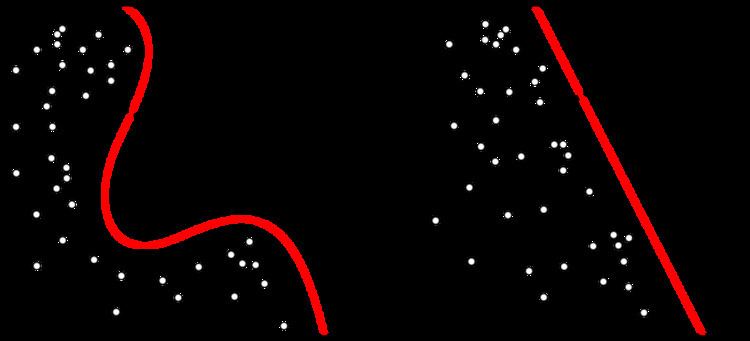
Nonlinear classification

The original maximum-margin hyperplane algorithm proposed by Vapnik in 1963 constructed a linear classifier. However, in 1992, Bernhard E. Boser, Isabelle M. Guyon and Vladimir N. Vapnik suggested a way to create nonlinear classifiers by applying the kernel trick (originally proposed by Aizerman et al.) to maximum-margin hyperplanes. The resulting algorithm is formally similar, except that every dot product is replaced by a nonlinear kernel function. This allows the algorithm to fit the maximum-margin hyperplane in a transformed feature space. The transformation may be nonlinear and the transformed space high dimensional; although the classifier is a hyperplane in the transformed feature space, it may be nonlinear in the original input space.

It is noteworthy that working in a higher-dimensional feature space increases the generalization error of support vector machines, although given enough samples the algorithm still performs well.

Some common kernels include:

The kernel is related to the transform φ ( x i → ) by the equation k ( x i → , x j → ) = φ ( x i → ) ⋅ φ ( x j → ) . The value w is also in the transformed space, with w → = ∑ i α i y i φ ( x → i ) . Dot products with w for classification can again be computed by the kernel trick, i.e. w → ⋅ φ ( x → ) = ∑ i α i y i k ( x → i , x → ) .

Computing the SVM classifier

Computing the (soft-margin) SVM classifier amounts to minimizing an expression of the form

We focus on the soft-margin classifier since, as noted above, choosing a sufficiently small value for λ yields the hard-margin classifier for linearly classifiable input data. The classical approach, which involves reducing (2) to a quadratic programming problem, is detailed below. Then, more recent approaches such as sub-gradient descent and coordinate descent will be discussed.

Primal

Minimizing (2) can be rewritten as a constrained optimization problem with a differentiable objective function in the following way.

For each i ∈ { 1 , … , n } we introduce a variable ζ i = max ( 0 , 1 − y i ( w ⋅ x i + b ) ) . Note that ζ i is the smallest nonnegative number satisfying y i ( w ⋅ x i + b ) ≥ 1 − ζ i .

Thus we can rewrite the optimization problem as follows

This is called the primal problem.

Dual

By solving for the Lagrangian dual of the above problem, one obtains the simplified problem

This is called the dual problem. Since the dual maximization problem is a quadratic function of the c i subject to linear constraints, it is efficiently solvable by quadratic programming algorithms.

Here, the variables c i are defined such that

Moreover, c i = 0 exactly when x → i lies on the correct side of the margin, and 0 < c i < ( 2 n λ ) − 1 when x → i lies on the margin's boundary. It follows that w → can be written as a linear combination of the support vectors.

The offset, b , can be recovered by finding an x → i on the margin's boundary and solving

(Note that y i − 1 = y i since y i = ± 1 .)

Kernel trick

Suppose now that we would like to learn a nonlinear classification rule which corresponds to a linear classification rule for the transformed data points φ ( x → i ) . Moreover, we are given a kernel function k which satisfies k ( x → i , x → j ) = φ ( x → i ) ⋅ φ ( x → j ) .

We know the classification vector w → in the transformed space satisfies

where the c i are obtained by solving the optimization problem

The coefficients c i can be solved for using quadratic programming, as before. Again, we can find some index i such that 0 < c i < ( 2 n λ ) − 1 , so that φ ( x → i ) lies on the boundary of the margin in the transformed space, and then solve

Finally, new points can be classified by computing

Modern methods

Recent algorithms for finding the SVM classifier include sub-gradient descent and coordinate descent. Both techniques have proven to offer significant advantages over the traditional approach when dealing with large, sparse datasets—sub-gradient methods are especially efficient when there are many training examples, and coordinate descent when the dimension of the feature space is high.

Sub-gradient descent

Sub-gradient descent algorithms for the SVM work directly with the expression

Note that f is a convex function of w → and b . As such, traditional gradient descent (or SGD) methods can be adapted, where instead of taking a step in the direction of the functions gradient, a step is taken in the direction of a vector selected from the function's sub-gradient. This approach has the advantage that, for certain implementations, the number of iterations does not scale with n , the number of data points.

Coordinate descent

Coordinate descent algorithms for the SVM work from the dual problem

For each i ∈ { 1 , … , n } , iteratively, the coefficient c i is adjusted in the direction of ∂ f / ∂ c i . Then, the resulting vector of coefficients ( c 1 ′ , … , c n ′ ) is projected onto the nearest vector of coefficients that satisfies the given constraints. (Typically Euclidean distances are used.) The process is then repeated until a near-optimal vector of coefficients is obtained. The resulting algorithm is extremely fast in practice, although few performance guarantees have been proven.

Empirical risk minimization

The soft-margin support vector machine described above is an example of an empirical risk minimization (ERM) algorithm for the hinge loss. Seen this way, support vector machines belong to a natural class of algorithms for statistical inference, and many of its unique features are due to the behavior of the hinge loss. This perspective can provide further insight into how and why SVMs work, and allow us to better analyze their statistical properties.

Risk minimization

In supervised learning, one is given a set of training examples X 1 … X n with labels y 1 … y n , and wishes to predict y n + 1 given X n + 1 . To do so one forms a hypothesis, f , such that f ( X n + 1 ) is a "good" approximation of y n + 1 . A "good" approximation is usually defined with the help of a loss function, ℓ ( y , z ) , which characterizes how bad z is as a prediction of y . We would then like to choose a hypothesis that minimizes the expected risk:

In most cases, we don't know the joint distribution of X n + 1 , y n + 1 outright. In these cases, a common strategy is to choose the hypothesis that minimizes the empirical risk:

Under certain assumptions about the sequence of random variables X k , y k (for example, that they are generated by a finite Markov process), if the set of hypotheses being considered is small enough, the minimizer of the empirical risk will closely approximate the minimizer of the expected risk as n grows large. This approach is called empirical risk minimization, or ERM.

Regularization and stability

In order for the minimization problem to have a well-defined solution, we have to place constraints on the set H of hypotheses being considered. If H is a normed space (as is the case for SVM), a particularly effective technique is to consider only those hypotheses f for which ∥ f ∥ H < k . This is equivalent to imposing a regularization penalty R ( f ) = λ k ∥ f ∥ H , and solving the new optimization problem

f ^ = a r g min f ∈ H ε ^ ( f ) + R ( f ) .

This approach is called Tikhonov regularization.

More generally, R ( f ) can be some measure of the complexity of the hypothesis f , so that simpler hypotheses are preferred.

SVM and the hinge loss

Recall that the (soft-margin) SVM classifier w ^ , b : x ↦ sgn ⁡ ( w ^ ⋅ x + b ) is chosen to minimize the following expression.

[ 1 n ∑ i = 1 n max ( 0 , 1 − y i ( w ⋅ x i + b ) ) ] + λ ∥ w ∥ 2

In light of the above discussion, we see that the SVM technique is equivalent to empirical risk minimization with Tikhonov regularization, where in this case the loss function is the hinge loss

From this perspective, SVM is closely related to other fundamental classification algorithms such as regularized least-squares and logistic regression. The difference between the three lies in the choice of loss function: regularized least-squares amounts to empirical risk minimization with the square-loss, ℓ s q ( y , z ) = ( y − z ) 2 ; logistic regression employs the log-loss, ℓ log ( y , z ) = ln ⁡ ( 1 + e − y z ) .

Target functions

The difference between the hinge loss and these other loss functions is best stated in terms of target functions - the function that minimizes expected risk for a given pair of random variables X , y .

In particular, let y x denote y conditional on the event that X = x . In the classification setting, we have:

The optimal classifier is therefore:

f ∗ ( x ) = { 1 if  p x ≥ 1 / 2 − 1 otherwise

For the square-loss, the target function is the conditional expectation function, f s q ( x ) = E [ y x ] ; For the logistic loss, it's the logit function, f log ⁡ ( x ) = ln ⁡ ( p x / ( 1 − p x ) ) . While both of these target functions yield the correct classifier, as sgn ⁡ ( f s q ) = sgn ⁡ ( f log ) = f ∗ , they give us more information than we need. In fact, they give us enough information to completely describe the distribution of y x .

On the other hand, one can check that the target function for the hinge loss is exactly f ∗ . Thus, in a sufficiently rich hypothesis space—or equivalently, for an appropriately chosen kernel—the SVM classifier will converge to the simplest function (in terms of R ) that correctly classifies the data. This extends the geometric interpretation of SVM—for linear classification, the empirical risk is minimized by any function whose margins lie between the support vectors, and the simplest of these is the max-margin classifier.

Properties

SVMs belong to a family of generalized linear classifiers and can be interpreted as an extension of the perceptron. They can also be considered a special case of Tikhonov regularization. A special property is that they simultaneously minimize the empirical classification error and maximize the geometric margin; hence they are also known as maximum margin classifiers.

A comparison of the SVM to other classifiers has been made by Meyer, Leisch and Hornik.

Parameter selection

The effectiveness of SVM depends on the selection of kernel, the kernel's parameters, and soft margin parameter C. A common choice is a Gaussian kernel, which has a single parameter γ . The best combination of C and γ is often selected by a grid search with exponentially growing sequences of C and γ , for example, C ∈ { 2 − 5 , 2 − 3 , … , 2 13 , 2 15 } ; γ ∈ { 2 − 15 , 2 − 13 , … , 2 1 , 2 3 } . Typically, each combination of parameter choices is checked using cross validation, and the parameters with best cross-validation accuracy are picked. Alternatively, recent work in Bayesian optimization can be used to select C and γ , often requiring the evaluation of far fewer parameter combinations than grid search. The final model, which is used for testing and for classifying new data, is then trained on the whole training set using the selected parameters.

Issues

Potential drawbacks of the SVM include the following aspects:

Support vector clustering (SVC)

SVC is a similar method that also builds on kernel functions but is appropriate for unsupervised learning and data-mining. It is considered a fundamental method in data science.

Multiclass SVM

Multiclass SVM aims to assign labels to instances by using support vector machines, where the labels are drawn from a finite set of several elements.

The dominant approach for doing so is to reduce the single multiclass problem into multiple binary classification problems. Common methods for such reduction include:

Crammer and Singer proposed a multiclass SVM method which casts the multiclass classification problem into a single optimization problem, rather than decomposing it into multiple binary classification problems. See also Lee, Lin and Wahba.

Transductive support vector machines

Transductive support vector machines extend SVMs in that they could also treat partially labeled data in semi-supervised learning by following the principles of transduction. Here, in addition to the training set D , the learner is also given a set

of test examples to be classified. Formally, a transductive support vector machine is defined by the following primal optimization problem:

Minimize (in w → , b , y ⋆ → )

subject to (for any i = 1 , … , n and any j = 1 , … , k )

and

Transductive support vector machines were introduced by Vladimir N. Vapnik in 1998.

Structured SVM

SVMs have been generalized to structured SVMs, where the label space is structured and of possibly infinite size.

Regression

A version of SVM for regression was proposed in 1996 by Vladimir N. Vapnik, Harris Drucker, Christopher J. C. Burges, Linda Kaufman and Alexander J. Smola. This method is called support vector regression (SVR). The model produced by support vector classification (as described above) depends only on a subset of the training data, because the cost function for building the model does not care about training points that lie beyond the margin. Analogously, the model produced by SVR depends only on a subset of the training data, because the cost function for building the model ignores any training data close to the model prediction. Another SVM version known as least squares support vector machine (LS-SVM) has been proposed by Suykens and Vandewalle.

Training the original SVR means solving

where x i is a training sample with target value y i . The inner product plus intercept ⟨ w , x i ⟩ + b is the prediction for that sample, and ε is a free parameter that serves as a threshold: all predictions have to be within an ε range of the true predictions. Slack variables are usually added into the above to allow for errors and to allow approximation in the case the above problem is infeasible.

Implementation

The parameters of the maximum-margin hyperplane are derived by solving the optimization. There exist several specialized algorithms for quickly solving the QP problem that arises from SVMs, mostly relying on heuristics for breaking the problem down into smaller, more-manageable chunks.

Another approach is to use an interior point method that uses Newton-like iterations to find a solution of the Karush–Kuhn–Tucker conditions of the primal and dual problems. Instead of solving a sequence of broken down problems, this approach directly solves the problem altogether. To avoid solving a linear system involving the large kernel matrix, a low rank approximation to the matrix is often used in the kernel trick.

Another common method is Platt's sequential minimal optimization (SMO) algorithm, which breaks the problem down into 2-dimensional sub-problems that are solved analytically, eliminating the need for a numerical optimization algorithm and matrix storage. This algorithm is conceptually simple, easy to implement, generally faster, and has better scaling properties for difficult SVM problems.

The special case of linear support vector machines can be solved more efficiently by the same kind of algorithms used to optimize its close cousin, logistic regression; this class of algorithms includes sub-gradient descent (e.g., PEGASOS) and coordinate descent (e.g., LIBLINEAR). LIBLINEAR has some attractive training time properties. Each convergence iteration takes time linear in the time taken to read the train data and the iterations also have a Q-Linear Convergence property, making the algorithm extremely fast.

The general kernel SVMs can also be solved more efficiently using sub-gradient descent (e.g. P-packSVM), especially when parallelization is allowed.

Kernel SVMs are available in many machine learning toolkits, including LIBSVM, MATLAB, SAS, SVMlight, kernlab, scikit-learn, Shogun, Weka, Shark, JKernelMachines, OpenCV and others.