Multivariate interpolation

Regular grid

For function values known on a regular grid (having predetermined, not necessarily uniform, spacing), the following methods are available.

Any dimension

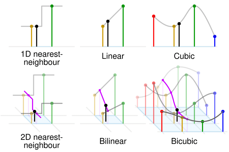
2 dimensions

Bitmap resampling is the application of 2D multivariate interpolation in image processing.

Three of the methods applied on the same dataset, from 16 values located at the black dots. The colours represent the interpolated values.

See also Padua points, for polynomial interpolation in two variables.

3 dimensions

See also bitmap resampling.

Tensor product splines for N dimensions

Catmull-Rom splines can be easily generalized to any number of dimensions. The cubic Hermite spline article will remind you that C I N T x ( f − 1 , f 0 , f 1 , f 2 ) = b ( x ) ⋅ ( f − 1 f 0 f 1 f 2 ) for some 4-vector b ( x ) which is a function of x alone, where f j is the value at j of the function to be interpolated. Rewrite this approximation as

This formula can be directly generalized to N dimensions:

Note that similar generalizations can be made for other types of spline interpolations, including Hermite splines. In regards to efficiency, the general formula can in fact be computed as a composition of successive C I N T -type operations for any type of tensor product splines, as explained in the tricubic interpolation article. However, the fact remains that if there are n terms in the 1-dimensional C R -like summation, then there will be n N terms in the N -dimensional summation.

Irregular grid (scattered data)

Schemes defined for scattered data on an irregular grid should all work on a regular grid, typically reducing to another known method.