Polyharmonic spline

Definition

A polyharmonic spline is a linear combination of polyharmonic radial basis functions (RBFs) denoted by ϕ plus a polynomial term:

where

The polynomial with the coefficients v improves fitting accuracy for polyharmonic smoothing splines and also improves extrapolation away from the centers c i . See figure below for comparison of splines with polynomial term and without polynomial term.

The polyharmonic RBFs are of the form:

Other values of the exponent k are not useful (such as ϕ ( r ) = r 2 ), because a solution of the interpolation problem might not exist. To avoid problems at r = 0 (since log ⁡ ( 0 ) = − ∞ ), the polyharmonic RBFs with the natural logarithm might be implemented as:

The weights w i and v j are determined such that the function interpolates N given points ( c i , f i ) (for i = 1 , 2 , … , N ) and fulfills the d + 1 orthogonality conditions

All together, these constraints are equivalent to the symmetric linear system of equations

where

In order for this system of equations to have a unique solution, B must be full rank. B is full rank for very mild conditions on the input data. For example, in two dimensions, three centers forming a non-degenerate triangle ensure that B is full rank, and in three dimensions, four centers forming a non-degenerate tetrahedron ensure that B is full rank. As explained later, the linear transformation resulting from the restriction of the domain of the linear transformation A to the null space of B T is positive definite. This means that if B is full rank, the system of equations (2) always has a unique solution and it can be solved using the Cholesky decomposition after a suitable transformation. The computed weights allow evaluation of the spline for any x ∈ R d using equation (1). Many practical details of implementing and using polyharmonic splines are explained in Fasshauer. In Iske polyharmonic splines are treated as special cases of other multiresolution methods in scattered data modelling.

Reason for the name "polyharmonic"

A polyharmonic equation is a partial differential equation of the form Δ m f = 0 for any natural number m . For example, the biharmonic equation is Δ 2 f = 0 and the triharmonic equation is Δ 3 f = 0 . All the polyharmonic radial basis functions are solutions of a polyharmonic equation (or more accurately, a modified polyharmonic equation with a Dirac delta function on the right hand side instead of 0). For example, the thin plate radial basis function is a solution of the modified 2-dimensional biharmonic equation. Applying the 2D Laplace operator ( Δ = ∂ x x + ∂ y y ) to the thin plate radial basis function f tp ( x , y ) = ( x 2 + y 2 ) log ⁡ x 2 + y 2 either by hand or using a computer algebra system shows that Δ f tp = 4 + 4 log ⁡ r . Applying the Laplace operator to Δ f tp (this is Δ 2 f tp ) yields 0. But 0 is not exactly correct. To see this, replace r 2 = x 2 + y 2 with ρ 2 = x 2 + y 2 + h 2 (where h is some small number tending to 0). The Laplace operator applied to 4 log ⁡ ρ yields Δ 2 f tp = 8 h 2 / ρ 4 . For ( x , y ) = ( 0 , 0 ) , the right hand side of this equation approaches infinity as h approaches 0. For any other ( x , y ) , the right hand side approaches 0 as h approaches 0. This indicates that the right hand side is a Dirac delta function. A computer algebra system will show that

So the thin plate radial basis function is a solution of the equation Δ 2 f tp = 8 π δ ( x , y ) .

Applying the 3D Laplacian ( Δ = ∂ x x + ∂ y y + ∂ z z ) to the biharmonic RBF f bi ( x , y , z ) = x 2 + y 2 + z 2 yields Δ f bi = 2 / r and applying the 3D Δ 2 operator to the triharmonic RBF f tri ( x , y , z ) = ( x 2 + y 2 + z 2 ) 3 / 2 yields Δ 2 f tri = 24 / r . Letting ρ 2 = x 2 + y 2 + z 2 + h 2 and computing Δ ( 1 / ρ ) = − 3 h 2 / ρ 5 again indicates that the right hand side of the PDEs for the biharmonic and triharmonic RBFs are Dirac delta functions. Since

the exact PDEs satisfied by the biharmonic and triharmonic RBFs are Δ 2 f bi = − 8 π δ ( x , y , z ) and Δ 3 f tri = − 96 π δ ( x , y , z ) .

Polyharmonic smoothing splines

Polyharmonic splines minimize

where B is some box in R d containing a neighborhood of all the centers, λ is some positive constant, and ∇ m f is the vector of all m th order partial derivatives of f . For example, in 2D ∇ 1 f = ( f x   f y ) and ∇ 2 f = ( f x x   f x y   f y x   f y y ) and in 3D ∇ 2 f = ( f x x   f x y   f x z   f y x   f y y   f y z   f z x   f z y   f z z ) . In 2D | ∇ 2 f | 2 = f x x 2 + 2 f x y 2 + f y y 2 , making the integral the simplified thin plate energy functional.

To show that polyharmonic splines minimize equation (3), the fitting term must be transformed into an integral using the definition of the Dirac delta function:

So equation (3) can be written as the functional

where α i is a multi-index that ranges over all partial derivatives of order m for R d . In order to apply the Euler-Lagrange equation for a single function of multiple variables and higher order derivatives, the quantities

and

are needed. Inserting these quantities into the E-L equation shows that

A weak solution f ( x ) of (4) satisfies

for all smooth test functions g that vanish outside of B . A weak solution of equation (4) will still minimize (3) while getting rid of the delta function through integration.

Let f be a polyharmonic spline as defined by equation (1). The following calculations will show that f satisfies (5). Applying the Δ m operator to equation (1) yields

where C 2 , 2 = 8 π , C 2 , 3 = − 8 π , and C 3 , 3 = − 96 π . So (5) is equivalent to

The only possible solution to (6) for all test functions g is

(which implies interpolation if λ = 0 ). Combining the definition of f in equation (1) with equation (7) results in almost the same linear system as equation (2) except that the matrix A is replaced with A + ( − 1 ) m C m , d λ I where I is the N × N identity matrix. For example, for the 3D triharmonic RBFs, A is replaced with A + 96 π λ I .

Explanation of additional constraints

In (2), the bottom half of the system of equations ( B T w = 0 ) is given without explanation. The explanation first requires deriving a simplified form of ∫ B | ∇ m f | 2 d x when B is all of R d .

First, require that ∑ i = 1 N w i = 0. This ensures that all derivatives of order m and higher of f ( x ) = ∑ i = 1 N w i ϕ ( | x − c i | ) vanish at infinity. For example, let m = 3 and d = 3 and ϕ be the triharmonic RBF. Then ϕ z z y = 3 y ( x 2 + y 2 ) / ( x 2 + y 2 + z 2 ) 3 / 2 (considering ϕ as a mapping from R 3 to R ). For a given center P = ( P 1 , P 2 , P 3 ) ,

On a line x = a + t b for arbitrary point a and unit vector b ,

Dividing both numerator and denominator of this by t 3 shows that lim t → ∞ ϕ z y y ( x − P ) = 3 b 2 ( b 2 2 + b 1 2 ) / ( b 1 2 + b 2 2 + b 3 2 ) 3 / 2 , a quantity independent of the center P . So on the given line,

It is not quite enough to require that ∑ i = 1 N w i = 0 , because in what follows it is necessary for f α g β to vanish at infinity, where α and β are multi-indices such that | α | + | β | = 2 m − 1. For triharmonic ϕ , w i u j ϕ α ( x − c i ) ϕ β ( x − d j ) (where u j and d j are the weights and centers of g ) is always a sum of total degree 5 polynomials in x , y , and z divided by the square root of a total degree 8 polynomial. Consider the behavior of these terms on the line x = a + t b as t approaches infinity. The numerator is a degree 5 polynomial in t . Dividing numerator and denominator by t 4 leaves the degree 4 and 5 terms in the numerator and a function of b only in the denominator. A degree 5 term divided by t 4 is a product of five b coordinates and t . The ∑ w = 0 (and ∑ u = 0 ) constraint makes this vanish everywhere on the line. A degree 4 term divided by t 4 is either a product of four b coordinates and an a coordinate or a product of four b coordinates and a single c i or d j coordinate. The ∑ w = 0 constraint makes the first type of term vanish everywhere on the line. The additional constraints ∑ i = 1 N w i c i = 0 will make the second type of term vanish.

Now define the inner product of two functions f , g : R d → R defined as a linear combination of polyharmonic RBFs ϕ m , d with ∑ w = 0 and ∑ w c = 0 as

Integration by parts shows that

For example, let m = 2 and d = 2. Then

Integrating the first term of this by parts once yields

since f x g x x vanishes at infinity. Integrating by parts again results in ∫ − ∞ ∞ ∫ − ∞ ∞ f g x x x x d x d y .

So integrating by parts twice for each term of (9) yields

Since ( Δ m f ) ( x ) = ∑ i = 1 N w i C m , d δ ( x − c i ) , (8) shows that

So if ∑ w = 0 and ∑ w c = 0 ,

Now the origin of the constraints B T w = 0 can be explained. Here B is a generalization of the B defined above to possibly include monomials up to degree m − 1. In other words,

B = [ 1 1 … 1 c 1 c 2 … c N ⋮ ⋮ … ⋮ c 1 m − 1 c 2 m − 1 … c N m − 1 ] T

where c i j is a column vector of all degree j monomials of the coordinates of c i . The top half of (2) is equivalent to A w + B v − f = 0. So to obtain a smoothing spline, one should minimize the scalar field F : R N + d + 1 → R defined by

The equations

and

(where A i ∗ denotes row i of A ) are equivalent to the two systems of linear equations A ( A w + B v − f + λ C w ) = 0 and B T ( A w + B v − f ) = 0. Since A is invertible, the first system is equivalent to A w + B v − f + λ C w = 0. So the first system implies the second system is equivalent to B T w = 0. Just as in the previous smoothing spline coefficient derivation, the top half of (2) becomes ( A + λ C I ) w + B v = f .

This derivation of the polyharmonic smoothing spline equation system did not assume the constraints necessary to guarantee that ∫ R d | ∇ m f | 2 d x = C w T A w . But the constraints necessary to guarantee this, ∑ w = 0 and ∑ w c = 0 , are a subset of B T w = 0 which is true for the critical point w of F . So ∫ R d | ∇ m f | 2 d x = C w T A w is true for the f formed from the solution of the polyharmonic smoothing spline equation system. Because the integral is positive for all w ≠ 0 , the linear transformation resulting from the restriction of the domain of linear transformation A to w such that B T w = 0 must be positive definite. This fact enables transforming the polyharmonic smoothing spline equation system to a symmetric positive definite system of equations that can be solved twice as fast using the Cholesky decomposition.

Examples

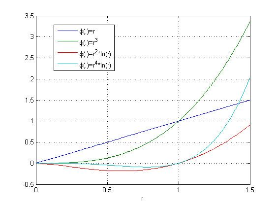
The next figure shows the interpolation through four points (marked by "circles") using different types of polyharmonic splines. The "curvature" of the interpolated curves grows with the order of the spline and the extrapolation at the left boundary (x < 0) is reasonable. The figure also includes the radial basis functions phi = exp(-r²) which gives a good interpolation as well. Finally, the figure includes also the non-polyharmonic spline phi = r² to demonstrate, that this radial basis function is not able to pass through the predefined points (the linear equation has no solution and is solved in a least squares sense).

The next figure shows the same interpolation as in the first figure, with the only exception that the points to be interpolated are scaled by a factor of 100 (and the case phi = r² is no longer included). Since phi = (scale*r)^k = (scale^k)*r^k, the factor (scale^k) can be extracted from matrix A of the linear equation system and therefore the solution is not influenced by the scaling. This is different for the logarithmic form of the spline, although the scaling has not much influence. This analysis is reflected in the figure, where the interpolation shows not much differences. Note, for other radial basis functions, such as phi = exp(-k*r²) with k=1, the interpolation is no longer reasonable and it would be necessary to adapt k.

The next figure shows the same interpolation as in the first figure, with the only exception that the polynomial term of the function is not taken into account (and the case phi = r² is no longer included). As can be seen from the figure, the extrapolation for x < 0 is no longer as "natural" as in the first figure for some of the basis functions. This indicates, that the polynomial term is useful if extrapolation occurs.

Discussion

The main advantage of polyharmonic spline interpolation is that usually very good interpolation results are obtained for scattered data without performing any "tuning", so automatic interpolation is feasible. This is not the case for other radial basis functions. For example, the Gaussian function e − k ⋅ r 2 needs to be tuned, so that k is selected according to the underlying grid of the independent variables. If this grid is non-uniform, a proper selection of k to achieve a good interpolation result is difficult or impossible.

Main disadvantages are:

Recently, methods have been developed to overcome the aforementioned difficulties. For example Beatson et al. present a method to interpolate polyharmonic splines at one point in 3 dimensions in O ( log ⁡ N ) operations instead of O ( N ) operations.