Cubic Hermite spline - Alchetron, The Free Social Encyclopedia

In numerical analysis, a cubic Hermite spline or cubic Hermite interpolator is a spline where each piece is a third-degree polynomial specified in Hermite form: that is, by its values and first derivatives at the end points of the corresponding domain interval.

Cubic Hermite splines are typically used for interpolation of numeric data specified at given argument values x 1 , x 2 , … , x n , to obtain a smooth continuous function. The data should consist of the desired function value and derivative at each x k . (If only the values are provided, the derivatives must be estimated from them.) The Hermite formula is applied to each interval ( x k , x k + 1 ) separately. The resulting spline will be continuous and will have continuous first derivative.

Cubic polynomial splines can be specified in other ways, the Bézier form being the most common. However, these two methods provide the same set of splines, and data can be easily converted between the Bézier and Hermite forms; so the names are often used as if they were synonymous.

Cubic polynomial splines are extensively used in computer graphics and geometric modeling to obtain curves or motion trajectories that pass through specified points of the plane or three-dimensional space. In these applications, each coordinate of the plane or space is separately interpolated by a cubic spline function of a separate parameter t.

Cubic splines can be extended to functions of two or more parameters, in several ways. Bicubic splines (Bicubic interpolation) are often used to interpolate data on a regular rectangular grid, such as pixel values in a digital image or altitude data on a terrain. Bicubic surface patches, defined by three bicubic splines, are an essential tool in computer graphics.

Cubic splines are often called csplines, especially in computer graphics. Hermite splines are named after Charles Hermite.

Unit interval (0, 1)

On the unit interval ( 0 , 1 ) , given a starting point p 0 at t = 0 and an ending point p 1 at t = 1 with starting tangent m 0 at t = 0 and ending tangent m 1 at t = 1 , the polynomial can be defined by

p ( t ) = ( 2 t 3 − 3 t 2 + 1 ) p 0 + ( t 3 − 2 t 2 + t ) m 0 + ( − 2 t 3 + 3 t 2 ) p 1 + ( t 3 − t 2 ) m 1

where t ∈ [0, 1].

Interpolation on an arbitrary interval

Interpolating x in an arbitrary interval ( x k , x k + 1 ) is done by mapping the latter to [ 0 , 1 ] through an affine (degree 1) change of variable. The formula is

p ( x ) = h 00 ( t ) p k + h 10 ( t ) ( x k + 1 − x k ) m k + h 01 ( t ) p k + 1 + h 11 ( t ) ( x k + 1 − x k ) m k + 1 .

with t = ( x − x k ) / ( x k + 1 − x k ) and h refers to the basis functions, defined below. Note that the tangent values have been scaled by x k + 1 − x k compared to the equation on the unit interval.

Uniqueness

The formulae specified above provide the unique third-degree polynomial path between the two points with the given tangents.
Proof:
Let Q ( x ) be another third degree polynomial satisfying the given boundary conditions. Define R ( x ) = Q ( x ) − P ( x ) . Since both Q and P are third degree polynomials, R is at most a third degree polynomial. Furthermore:

R ( 0 ) = Q ( 0 ) − P ( 0 ) = 0 (We assume both P and Q satisfy the boundary conditions) R ( 1 ) = 0

So R must be of the form:

R ( x ) = a x ( x − 1 ) ( x − r ) R ′ ( x ) = a x ( x − 1 ) + a x ( x − r ) + a ( x − 1 ) ( x − r )

We know furthermore that:

R ′ ( 0 ) = Q ′ ( 0 ) − P ′ ( 0 ) = 0 R ′ ( 1 ) = Q ′ ( 1 ) − P ′ ( 1 ) = 0

Putting (1) and (2) together, we deduce that a = 0 and therefore R = 0 , thus P ( x ) = Q ( x )

Representations

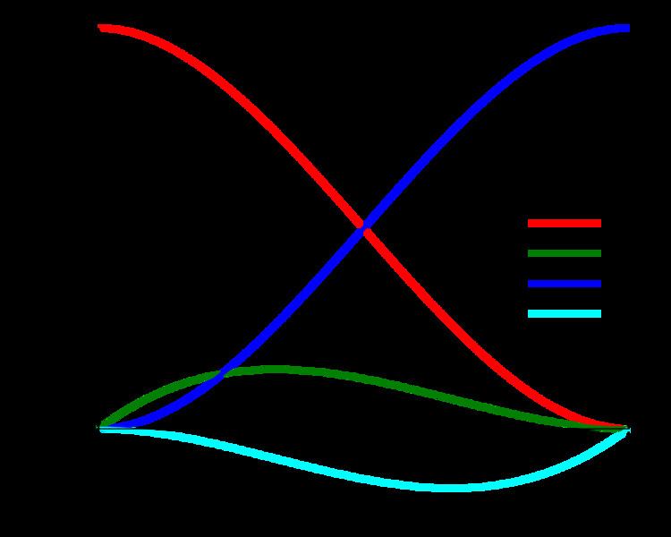
We can write the interpolation polynomial as

p ( t ) = h 00 ( t ) p 0 + h 10 ( t ) m 0 + h 01 ( t ) p 1 + h 11 ( t ) m 1

where h 00 , h 10 , h 01 , h 11 are Hermite basis functions. These can be written in different ways, each way revealing different properties.

The "expanded" column shows the representation used in the definition above. The "factorized" column shows immediately, that h 10 and h 11 are zero at the boundaries. You can further conclude that h 01 and h 11 have a zero of multiplicity 2 at 0 and h 00 and h 10 have such a zero at 1, thus they have slope 0 at those boundaries. The "Bernstein" column shows the decomposition of the Hermite basis functions into Bernstein polynomials of order 3:

B k ( t ) = ( 3 k ) ⋅ t k ⋅ ( 1 − t ) 3 − k

Using this connection you can express cubic Hermite interpolation in terms of cubic Bézier curves with respect to the four values p 0 , p 0 + m 0 3 , p 1 − m 1 3 , p 1 and do Hermite interpolation using the de Casteljau algorithm. It shows that in a cubic Bézier patch the two control points in the middle determine the tangents of the interpolation curve at the respective outer points.

Interpolating a data set

A data set, ( t k , p k ) for k = 1 , … , n , can be interpolated by applying the above procedure on each interval, where the tangents are chosen in a sensible manner, meaning that the tangents for intervals sharing endpoints are equal. The interpolated curve then consists of piecewise cubic Hermite splines, and is globally continuously differentiable in ( t 1 , t n ) .

The choice of tangents is non-unique, and there are several options available.

Finite difference

The simplest choice is the three-point difference, not requiring constant interval lengths,

m k = 1 2 ( p k + 1 − p k t k + 1 − t k + p k − p k − 1 t k − t k − 1 )

for internal points k = 2 , … , n − 1 , and one-sided difference at the endpoints of the data set.

Cardinal spline

A cardinal spline, sometimes called a canonical spline, is obtained if

m k = ( 1 − c ) p k + 1 − p k − 1 t k + 1 − t k − 1

is used to calculate the tangents. The parameter c is a tension parameter that must be in the interval [0,1]. In some sense, this can be interpreted as the "length" of the tangent. Choosing c=1 yields all zero tangents, and choosing c=0 yields a Catmull–Rom spline.

Catmull–Rom spline

For tangents chosen to be

m n = p n + 1 − p n − 1 t n + 1 − t n − 1

a Catmull–Rom spline is obtained, being a special case of a cardinal spline. This assumes uniform parameter spacing.

The curve is named after Edwin Catmull and Raphael Rom. The principal advantage of this technique is that the points along the original set of points also make up the control points for the spline curve. Two additional points are required on either end of the curve. The default implementation of the Catmull–Rom algorithm can produce loops and self intersections. The chordal and centripetal Catmull–Rom implementations solve this problem, but use a slightly different calculation. In computer graphics, Catmull–Rom splines are frequently used to get smooth interpolated motion between key frames. For example, most camera path animations generated from discrete key-frames are handled using Catmull–Rom splines. They are popular mainly for being relatively easy to compute, guaranteeing that each key frame position will be hit exactly, and also guaranteeing that the tangents of the generated curve are continuous over multiple segments.

Kochanek–Bartels spline

A Kochanek–Bartels spline is a further generalization on how to choose the tangents given the data points p k − 1 , p k and p k + 1 , with three parameters possible, tension, bias and a continuity parameter.

Monotone cubic interpolation

If a cubic Hermite spline of any of the above listed types is used for interpolation of a monotonic data set, the interpolated function will not necessarily be monotonic, but monotonicity can be preserved by adjusting the tangents.

Interpolation on the unit interval with matched derivatives at endpoints

Considering a single coordinate of the points p n − 1 , p n , p n + 1 and p n + 2 as the values that a function, f(x), takes at integer ordinates x=n−1, n, n+1 and n+2,

p n = f ( n ) ∀ n ∈ Z

If, in addition, the tangents at the endpoints are defined as the centered differences of the adjacent points,

m n = f ( n + 1 ) − f ( n − 1 ) 2 = p n + 1 − p n − 1 2 ∀ n ∈ Z

To evaluate the interpolated f(x) for a real x, first separate x into the integer portion, n, and fractional portion, u

x = n + u n = ⌊ x ⌋ = floor ⁡ ( x ) u = x − n = x − ⌊ x ⌋ 0 ≤ u < 1

Then the Catmull–Rom spline is

f ( x ) = f ( n + u ) = C I N T u ( p n − 1 , p n , p n + 1 , p n + 2 ) = [ 1 u u 2 u 3 ] ⋅ [ 0 1 0 0 − 1 2 0 1 2 0 1 − 5 2 2 − 1 2 − 1 2 3 2 − 3 2 1 2 ] ⋅ [ p n − 1 p n p n + 1 p n + 2 ] = 1 2 [ − u 3 + 2 u 2 − u 3 u 3 − 5 u 2 + 2 − 3 u 3 + 4 u 2 + u u 3 − u 2 ] T ⋅ [ p n − 1 p n p n + 1 p n + 2 ] = 1 2 [ u ( ( 2 − u ) u − 1 ) u 2 ( 3 u − 5 ) + 2 u ( ( 4 − 3 u ) u + 1 ) u 2 ( u − 1 ) ] T ⋅ [ p n − 1 p n p n + 1 p n + 2 ] = 1 2 ( ( u 2 ( 2 − u ) − u ) p n − 1 + ( u 2 ( 3 u − 5 ) + 2 ) p n + ( u 2 ( 4 − 3 u ) + u ) p n + 1 + u 2 ( u − 1 ) p n + 2 )

⌊ x ⌋ denotes the floor function which returns the largest integer no larger than x and T denotes the matrix transpose.

This writing is relevant for tricubic interpolation, where one optimization requires you to compute CINT_u sixteen times with the same u and different p.